
SLIDE 1
Hyperbolic Systems (spring 2001)
Hans De Sterck
Department of Applied Mathematics, CU Boulder
Introduction – motivation
- ✁
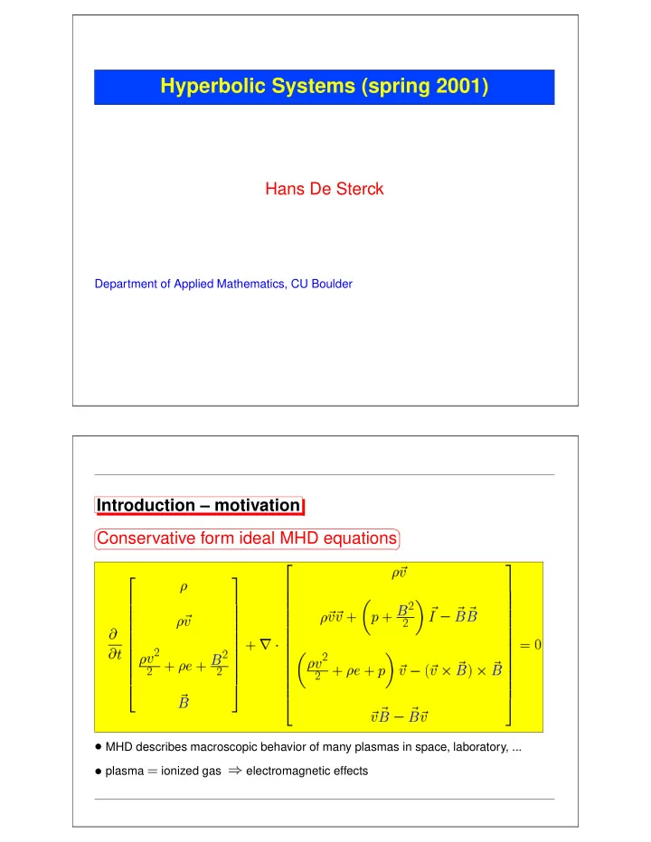
Hyperbolic Systems (spring 2001) Hans De Sterck Department of - - PDF document
(a) static (b) subsonic (c) supersonic
+ c v - c v + c v ( < c ) v ( > c ) v - c v + c v = 0
(b) shock (N-S) (a) continuous profile (c) shock (Euler) x δ
X Y Z "rho" 2.63673 2.43265 2.22857 2.02449 1.82041 1.61633 1.41224 1.20816 1.00408 0.8 X Y Z X Y Z X Y Z
(b) electron temperature (K)
16 17 18 19 20 Ulysses, February 2, 1992 (time in UT) 1.3•105 5.3•105 9.3•105 1.3•106
(a) magnetic field (nT)
16 17 18 19 20 1 2 3 4 5
0.1 1.0 10.0 100.0 β 8 10 12 14 M 10 100 MA 0.02 0.04 0.06 0.08 0.10 0.12 p (nPa) 0.05 0.10 0.15 0.20 0.25 pB (nPa) 0.1 0.2 0.3 ptot (nPa) 400 450 500 550 600 v (km/s) 50 100 150 θB 2 4 6 8 10 θv 0 hrs (9 Jan) 0 hrs (10 Jan) 0 hrs (11 Jan) 0 hrs (12 Jan)
10 20 Bz (nT)
cosmic rays galactic termination shock bow shock Voyager 2 Pioneer 10 Voyager 1 Pioneer 11 heliopause solar wind
(b) 0.0 0.5 1.0 0.0 0.5 1.0
0.5 1 1.5 t x u
1 u
0.333 f(u)
1 u 1 f ’(u)
u*
*
p p
l
1 (c) u 1 1
x
(b) t t x 1
(a) x 1
1
i-1 1
x
N-1
1 ∆x
N
x x x x x
✴ i+1 i-1
n n+1
i+1 i-1
i+1 i-1
n n+1
domain of dependency physical characteristics characteristics physical domain of dependency
✁ for systems: several wave speeds, domain of dependence delineated by characteristics i i+1 i-1 f(u )
i-1/2
f(u )
i+1/2
ui ui n+1 n t x
n+1 n n* n*
s u u u
r l
* x t
✴ ( i , j+1 ) ( i , j ) ( i+1 , j ) ( i , j-1 ) ( i-1 , j ) x y
(b) 0.0 0.5 1.0 0.0 0.5 1.0
0.5 1 1.5 t x u
8 16 24 32 processors 8 16 24 32 speedup