How do we remove aliasing ? Anti-Aliasing Techniques Cheaper - PDF document

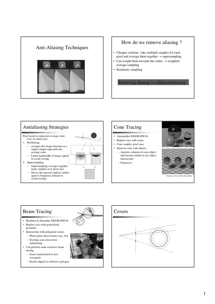
How do we remove aliasing ? Anti-Aliasing Techniques • Cheaper solution : take multiple samples for each pixel and average them together → supersampling. • Can weight them towards the centre → weighted average sampling • Stochastic sampling Removing aliasing is called antialiasing Antialiasing Strategies Cone Tracing Pixel needs to represent average color • Amanatides SIGGRAPH 84 over its entire area • Replace rays with cones 1. Prefiltering • Cone samples pixel area – averages the image function so a • Intersect cone with objects single sample represents the average color – Analytic solution of cone-object Prefiltering Supersampling intersection similar to ray-object – Limits bandwidth of image signal to avoid overlap intersection 2. Supersampling – Expensive – Supersampling averages together many samples over pixel area – Moves the spectral replicas farther apart in frequency domain to Images courtesy John Amanatides avoid overlap Beam Tracing Covers • Heckbert & Hanrahan SIGGRAPH 84 • Replace rays with generalized pyramids • Intersection with polygonal scenes – Plane-plane intersections easy, fast – Existing scan conversion antialiasing • Can perform some recursive beam tracing – Scene transformed to new viewpoint – Result clipped to reflective polygon 1

Supersampling Stochastic Sampling • Trace at higher resolution, average • Eye is extremely sensitive to patterns results • Remove pattern from sampling • Randomize sampling pattern • Adaptive supersampling • Result: patterns -> noise – trace at higher resolution only • Some noises better than others where necessary • Jitter : Pick n random points in sample space • Problems – Easiest, but samples cluster – Does not eliminate aliases (e.g. • Uniform Jitter : Subdivide sample space into n moire patterns) regions, and randomly sample in each region – Easier, but can still cluster – Makes aliases higher-frequency • Poisson Disk : Pick n random points, but not – Due to uniformity of samples too close to each other – Samples can’t cluster, but may run out of room Stochastic Sampling Stochastic Sampling Poisson Poisson Disc Jitter Analytic Area OpenGL Aliases Sampling • Aliasing due to rasterization • Ed Catmull, 1978 • Opposite of ray casting • Eliminates edge aliases • New polygons-to-pixels strategies • Clip polygon to pixel boundary • Prefiltering • Sort fragments by depth – Edge aliasing • Clip fragments against each other • Analytic Area Sampling • Scale color by visible area • A-Buffer • Sum scaled colors – Texture aliasing • MIP Mapping • Summed Area Tables • Postfiltering – Accumulation Buffer 2

A-Buffer Texture Aliasing • Loren Carpenter, 1984 • Image mapped onto polygon • Subdivides pixel into 4x4 bitmasks • Occur when screen resolution differs from texture resolution • Clipping = logical operations on bitmasks • Magnification aliasing • Bitmasks used as index to lookup table – Screen resolution finer than texture resolution – Multiple pixels per texel • Minification aliasing – Screen resolution coarser than texture resolution – Multiple texels per pixel Magnification Minification Filtering Filtering • Nearest neighbor • Multiple texels per pixel – Equivalent to spike filter • Potential for aliasing since texture signal bandwidth greater than framebuffer • Box filtering requires averaging of • Linear interpolation texels – Equivalent to box filter • Precomputation – MIP Mapping – Summed Area Tables MIP Mapping Summed Area Table x , y • Lance Williams, 1983 • Frank Crow, 1984 x -1, y -1 • Create a resolution pyramid of textures • Replaces texture map with summed-area texture map – Repeatedly subsample texture at half resolution – S ( x , y ) = sum of texels <= x , y – Until single pixel – Need double range (e.g. 16 bit) – Need extra storage space • Creation • Accessing – Incremental sweep using previous computations – Use texture resolution closest to – S ( x , y ) = T ( x , y ) + S ( x -1, y ) + S ( x , y -1) - S ( x -1, y -1) x 2 , y 2 screen resolution • Accessing – Or interpolate between two closest – Σ T ([ x 1 , x 2 ],[ y 1 , y 2 ]) = S ( x 2 , y 2 ) – S ( x 1 , y 2 ) – x 1 , y 1 resolutions S ( x 2 , y 1 ) + S ( x 1 , y 1 ) – Ave T ([ x 1 , x 2 ],[ y 1 , y 2 ])/(( x 2 – x 1 )( y 2 – y 1 )) 3

Accumulation Buffer Aliased vs. Antialiased • Increases OpenGL’s resolution • Render the scene 16 times • Shear projection matrices • Samples in different location in pixel • Average result • Jittered, but same jitter sampling pattern in each pixel Polygon Edges Line Antialising Polygon Antialising Close-up 4

Line Anti-aliasing Line Anti-aliasing Abram & Westover, 1983 Abram & Westover, 1983 4 הרקמל המגוד 3 הרקמל המגוד הרקמ 5 הרקמ 4 הרקמ 3 3 הרקמל המגוד 2 הרקמל SuperSampling Abram & Westover, 1983 Sample at 4x4 subpixels and color the pixel according to the portion of the coverage. 5

Andreas Schilling Andreas Schilling • • • • • • • • Andreas Schilling Texture Aliasing • A single screen space pixel might correspond to 0 1 2 3 many texels (texture elements): 4 5 6 7 8 9 10 11 12 13 14 15 12 8 4 0 13 9 5 1 14 10 6 2 15 11 7 3 Texture Mapping Two special cases: • Magnification: No real need in prefiltering. The main decision is what kind of reconstruction (interpolation) to use. • Minification: No real need in reconstruction. The main problem is proper prefiltering. 6

Nearest neighbor sampling Filtered Texture: Magnification Filtering Texture Pre-Filtering • Nearest neighbor – Equivalent to spike filter • Problem: filtering the texture during rendering is too slow for interactive performance. • Linear interpolation • Solution: pre-filter the texture in advance – Equivalent to box filter – Summed area tables - gives the average value of each axis-aligned rectangle in texture space – Mip-maps (tri-linear interpolation) - supported by most of today’s texture mapping hardware MI P Maps MIP-Maps • Precompute a set of prefiltered textures (essentially an image pyramid). • Based on the area of the pre-image of the pixel: – Select two “best” resolution levels – Use bilinear interpolation inside each level – Linearly interpolate the results • Referred to as trilinear interpolation 7

MIP Mapping Texture Aliasing • Lance Williams, 1983 • Image mapped onto polygon • Create a resolution pyramid of textures • Occur when screen resolution differs from texture – Repeatedly subsample texture at half resolution resolution – Until single pixel • Magnification aliasing – Need extra storage space • Accessing – Screen resolution finer than texture resolution – Use texture resolution closest to screen – Multiple pixels per texel resolution • Minification aliasing – Or interpolate between two closest – Screen resolution coarser than texture resolution resolutions – Multiple texels per pixel Summed Area Table Minification Filtering x , y • Frank Crow, 1984 x -1, y -1 • Replaces texture map with summed-area texture • Multiple texels per pixel map • Potential for aliasing since texture signal – S ( x , y ) = sum of texels <= x , y bandwidth greater than framebuffer – Need double range (e.g. 16 bit) • Creation • Box filtering requires averaging of texels – Incremental sweep using previous computations • Precomputation – S ( x , y ) = T ( x , y ) + S ( x -1, y ) + S ( x , y -1) - S ( x -1, y -1) x 2 , y 2 – MIP Mapping • Accessing – Σ T ([ x 1 , x 2 ],[ y 1 , y 2 ]) = S ( x 2 , y 2 ) – S ( x 1 , y 2 ) – – Summed Area Tables x 1 , y 1 S ( x 2 , y 1 ) + S ( x 1 , y 1 ) – Ave T ([ x 1 , x 2 ],[ y 1 , y 2 ])/(( x 2 – x 1 )( y 2 – y 1 )) Quality considerations Summed Area Tables • Pixel area maps to “ weird ” (warped) • A 2D table the size of the texture. At each shape in texture space entry (i,j), store the sum of all texels in the rectangle defined by (0,0) and (i,j). v • Given any axis aligned rectangle, the sum y s of all texels is easily obtained from the pixel summed area table: = − − + D D B B = − − + area area A A B B C C D D x s u C C A A 8

Mip-maps Summed Area Table (SAT) • Find level of the mip-map where the area of each • Determining the rectangle: mip-map pixel is closest to the area of the mapped – Find bounding box and calculate its aspect ratio pixel. v v y s y s pixel pixel x s u x s u 2x2 pixels level selected Elliptical Weighted Average Summed Area Table (SAT) (EWA) Filter • Determine the rectangle with the same aspect ratio • Treat each pixel as circular, rather than square. as the bounding box and the same area as the pixel • Mapping of a circle is elliptical in texel space. mapping. v y s y s pixel v pixel x s u x s u Elliptical Weighted Average Texture Domain 9

Accumulation Buffer tests • Increases OpenGL’s resolution • Render the scene 16 times • Shear projection matrices • Samples in different location in pixel • Average result • Jittered, but same jitter sampling pattern in each pixel 10