Homework Due date Tucker Rosen Mat 3770 4/7 4.1 9.6, set 1 - PDF document

Homework Due date Tucker Rosen Mat 3770 4/7 4.1 9.6, set 1 Week 11 4/7 Dijkstra–I worksheet 4/9 9.6, set 2 4/9 Dijkstra–II worksheet Spring 2014 4/11 3.4 10.5 4/11 TSP worksheet 1 2 Week 11 — More Student Responsibilities Single Source – Shortest Paths ◮ Problem Statement : Given a direct graph G = (V, E), with edge weights and a vertex v ∈ V, find the weight of a shortest path ◮ Reading, Tucker: 4.1, 3.4 from v to every other vertex in G. ◮ Reading, Rosen: 9.6, (653–655) ◮ Assumptions : ◮ Attendance Spring-i-ly Encouraged 1. Weights are positive real numbers ( w : E G → ℜ + ) 2. Path weights = sum of weights of all edges in the path 3. Define SHORT (w) to be the weight of the shortest path from v to w. 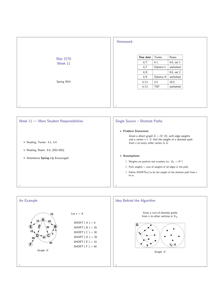3 4 An Example Idea Behind the Algorithm Grow a tree of shortest paths Let v = A 70 from v to other vertices in V G . A 10 50 SHORT ( A ) = 0 G 100 E B 30 SHORT ( B ) = 35 10 SHORT ( C ) = 30 v 5 D C SHORT ( D ) = 20 50 20 SHORT ( E ) = 10 20 F V − S S G SHORT ( F ) = 40 Graph G Graph G 5 6

Let S ⊆ V G , v ∈ S. Claim : Suppose for each w ∈ S , we know SHORT(w). If (w, u) is the edge minimizing SHORT(w) + weight(w, u) B — over all w ∈ S and u ∈ V - S — 50 (v) A V−S then 30 S G C SHORT(u) = SHORT(w) + weight(w, u) . 100 D F E 10 10 In other words, pick vertex from V - S to add to S which has the Graph G least weight path. For each (w, u) ∈ E g , where w ∈ S , u ∈ V G - S , look at SHORT(w) + weight(w,u) . Thus, we add u to S and (w, u) to the tree. 7 8 Proof: Consider (w, u) ◮ Observation : { v = v 1 , v 2 , . . . , v k − 1 } are all in S ! (Else there is a shorter path, ending before v k ). G v P v k−1 k v ◮ Hence weight( P ) = SHORT( v k − 1 ) + weight( v k − 1 , v k ) u ≥ SHORT(w) + weight(w, u) w V − S S G ◮ Thus, [ the shortest path from v to w ] + [ edge(w, u) ] Graph G gives a path from v to u which is as short as any path from v to any x ∈ V - S . Let P = { v = v 1 , v 2 , . . . , v k } be the least weight path from v to some vertex v k ∈ V - S . 9 10 Algorithm — First Pass SHORT(i) Dijkstra(G, v) : SHORT[1..n] Step S V-S A B C D E F // Initializations Init A BCDEF 0 ∞ ∞ ∞ ∞ ∞ S ← v 1 AE BCDF 0 ∞ ∞ ∞ 10 ∞ SHORT[v] ← 0 2 AED BCF 0 ∞ ∞ 20 10 ∞ FOR each w � = v do SHORT[w] ← ∞ 3 AEDC BF 0 ∞ 30 20 10 ∞ 4 AEDCB F 0 35 30 20 10 ∞ // Build tree of shortest paths While | S | < | V | do 5 AEDCBF 0 35 30 20 10 40 Find edge e = (w, u) such that w ∈ S, u ∈ V-S, and SHORT(w) + weight(w, u) is minimal SHORT(u) ← SHORT(w) + weight(w, u) We want to minimize SHORT(w) + weight(w, u). S ← S ∪ { u } 11 12

Implementation Analysis ◮ Then we could 1. search the list D for best u and add u to S 2. next we would update D, since D[u’] may have changed for some ◮ What are the slow steps — i.e., what will bound our time? elements Find edge e = (w, u) such that w ∈ S, u ∈ V-S, and ◮ So, how long to update D? SHORT(w) + weight(w, u) is minimal 1. Well, how many elements need changed? 2. At most, outdeg(u) vertices — the neighbors of u ◮ Thus, overall time updating D is: � u ∈ V outdeg ( u ) = | E | ◮ Suppose we had a TABLE, D[1..n], for u �∈ S, where: ◮ and, the algorithm takes time: D[u] = min w ∈ S { SHORT[w] + weight(w, u) } O ( | V | ∗ | V | + | E | ) = O ( | V | 2 + | E | ) or # iterations × Search D + Update D 13 14 Dijkstra(v) // v is the source node // Delete source from nodes not considered so far // and set distance to itself to 0 variables : V’ = V - { v } D[ ] — the length of the shortest path from v to each node D[v] = 0 P[ ] — the parent of each node // Determine shortest distances and parents // Initialize cost to each node from source for i = 1 to n − 1 // and make source the parent Select u ∈ V’ such that D[u] = min x ∈ V ′ D[x] for all vertices u ∈ V V’ = V’ − { u } for all w ∈ V’ if (v, u) ∈ E //Do we get shorter path to w through u? D[u] = weight(v, u) if D[w] > D[u] + weight(u, w) else D[w] = D[u] + weight (u,w) D[u] = ∞ P[w] = u P[u] = v 15 16 Obtaining Shortest Path Routes, source to sink Can We Do Better? We always want to find the minimum in D Idea : backtrack through parents until source is reached ◮ If we implement D as a min–heap, Searching takes O(1) time for all nodes w ∈ V // print shortest path from w to v ◮ But , how would we then update D? q = w I.e., when u is added to S, if (u, u’) ∈ E, u’ ∈ V-S, we may need print q to change D[u’] while q � = v q = P[q] ◮ Solution: Add a table , Dindex[1..n] which stores the position of print q vertices in heap D print q Whenever heap elements are moved, update Dindex[]. 17 18

The Traveling Salesperson Problem ◮ Now, updating D and Dindex takes outdeg(u) * log | V | steps ◮ Problem Statement : Given a graph, find the least–cost circuit which includes ◮ So the algorithm takes every vertex — i.e., the cheapest Hamilton Circuit. O (( | V | + | E | ) ∗ log | V | ) time ◮ Multiple Uses : ◮ Is this better than O ( | V | 2 + | E | ) 1. Business and industry, ex: robotic motion planning for wiring or laser–drilled holes in circuit boards ◮ Yes, if | E | ∈ O ( | V | 2 2. Efficient routing of telephone calls and Internet connections log | V | ) 3. Archaeologists: help in determining the sequence of deposits For example, if G is planar or not “almost complete” (i.e., sparse). 4. Delivery routes 19 20 Several algorithms TSP: Brute Force C D A B A D A D C 1. Brute Force B D A A C 2. Nearest Neighbor A D B B C B C A 3. Branch and Bound D C B A 4. Approximation Algorithm, Using Minimal Spanning Tree 1. Select a starting point 5. And others. . . 2. Enumerate all possible Hamilton Circuits with that starting point 3. Find the total weight of each circuit 4. choose one which produces the minimum cost 21 22 Brute Force Example Efficiency of Brute Force? ◮ The Brute Force method provides a way to find a minimum 3 A D Hamilton circuit if one exists (optimal solution). 1 4 1 6 ◮ Consider a complete, weighted graph with 10 vertices. How many circuits and total weights would we have to calculate for B this graph? (10!, or 3,628,800 Hamilton circuits, but we’d only C 3 have to calculate the weights for half of them. . . ) Total weight ◮ So, in worst case, if the graph had n vertices, how long would Circuit of the circuit this algorithm take to execute? Is that feasible? 1. A → B → C → D → A 3 + 6 + 3 + 1 = 13 2. A → B → D → C → A 3 + 4 + 3 + 1 = 11 ◮ If we used the Brute Force algorithm as the basis for a program 3. A → C → B → D → A 1 + 6 + 4 + 1 = 12 for a super–computer, and had fed it a 100–vertex TSP when 4. A → C → D → B → A (opp 2) 11 the universe was created, it would still be far from 5. A → D → B → C → A (opp 3) 12 done. . . (100! = 9 . 3326211544 × 10 157 ) 6. A → D → C → B → A (opp 1) 13 23 24

Approximation Algorithms Nearest Neighbor Algorithm Idea : choose as the next vertex, the nearest one to the current vertex. (Used on complete graphs.) 1. Choose a starting point for the circuit; say vertex A Algorithms which do not take too much computer time, 2. Check all the edges incident to A , and choose one that has and that give reasonably good solutions smallest weight; proceed along this edge to the next vertex most of the time are called 3. Repeat approximation algorithms . At each vertex you reach, check the edges from there to vertices not yet visited . Choose one with smallest weight. Proceed along this edge to the next vertex. until all vertices have been reached 4. Return to the starting vertex 25 26 Nearest Neighbor Example A courier is based at the head office (A), and must deliver documents to four other offices (B, C, D, and E). The estimated time of travel in minutes between each of these offices is shown on the graph below. Answer: A 9 20 Total Weight: 13 9 E B 3 Is this the optimum answer? 8 8 5 10 7 C D Use the Nearest Neighbor algorithm to find an approximate solution to this problem. Calculate the total time required to cover the chosen route. Begin at A. 27 28 The Branch and Bound Algorithm Starting Circuit Using Vertex Nearest Neighbor Total Weight A → D → E → B → C → A 9 + 5 + 3 + 10 + 13 = 40 A B → E → D → C → A → B 3 + 5 + 7 + 13 + 9 = 37 B A general and usually inefficient method for solving optimization C → D → E → B → A → C 7 + 5 + 3 + 9 + 13 = 37 problems. C D D → E → B → A → C → D 5 + 3 + 9 + 13 + 7 = 37 E E → B → D → C → A → E 3 + 8 + 7 + 13 + 20 = 51 Goal ◮ Any circuit of minimum weight may be used. Find the best (i.e., optimal) solution to a problem. Used for optimization problems and Artificial Intelligence ◮ Since these are circuits, may begin at any office. ◮ Have we found a minimum Hamilton Circuit? Optimality is not guaranteed with Approximation Algorithms. 29 30