[PPT] - h ( t ) x ( t ) y ( t ) x ( t ) y ( t ) H ( j ) CT Fourier Series as PowerPoint Presentation

SLIDE 1

CT Periodic Signals Design Task

1 2 1

1
2

t x(t)

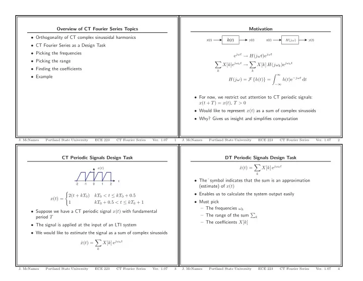
x(t) =

2(t + kT0)

kT0 < t ≤ kT0 + 0.5 1 kT0 + 0.5 < t ≤ kT0 + 1

Suppose we have a CT periodic signal x(t) with fundamental

period T

The signal is applied at the input of an LTI system
We would like to estimate the signal as a sum of complex sinusoids

ˆ x(t) =

k

X[k] ejωkt

J. McNames

Portland State University ECE 223 CT Fourier Series

Ver. 1.07

3

Overview of CT Fourier Series Topics

Orthogonality of CT complex sinusoidal harmonics
CT Fourier Series as a Design Task
Picking the frequencies
Picking the range
Finding the coefficients
Example
J. McNames

Portland State University ECE 223 CT Fourier Series

Ver. 1.07

1

DT Periodic Signals Design Task ˆ x(t) =

k

X[k] ejωkt

Theˆsymbol indicates that the sum is an approximation

(estimate) of x(t)

Enables us to calculate the system output easily
Must pick

– The frequencies ωk – The range of the sum

k

– The coefficients X[k]

J. McNames

Portland State University ECE 223 CT Fourier Series

Ver. 1.07

4

Motivation h(t)

x(t) y(t) x(t) y(t)

H(jω)

ejωt → H(jωt)ejωt

k

X[k]ejωkt →

k

X[k] H(jωk)ejωkt H(jω) = F {h(t)} = ∞

−∞

h(t)e−jωt dt

For now, we restrict out attention to CT periodic signals:

x(t + T) = x(t), T > 0

Would like to represent x(t) as a sum of complex sinusoids
Why? Gives us insight and simplifies computation
J. McNames

Portland State University ECE 223 CT Fourier Series

Ver. 1.07

2

SLIDE 2

Design Task: Picking the Coefficients ˆ x(t) =

∞

k=−∞

X[k] ejkωt MSE = 1 T

T

|x(t) − ˆ x(t)|2 dt

We would like to pick the coefficients X[k] so that ˆ

x(t) is as close to x(t) as possible

But what is close?
One measure of the difference between two signals is the mean

squared error (MSE)

There are other measures, but this is a convenient one because we

can differentiate it

If MSE = 0, does this imply x(t) = ˆ

x(t)?

Since the signal is periodic, the MSE is calculated over a single

fundamental period of T

How do we pick the coefficients X[k] to minimize the MSE?
J. McNames

Portland State University ECE 223 CT Fourier Series

Ver. 1.07

7

Design Task: Picking the Frequencies ˆ x(t) =

k

X[k] ejωkt

We know x(t) is periodic with some fundamental period T
If ˆ

x(t) is to approximate x(t) accurately, it should also repeat every T seconds

In order for ˆ

x(t) to be periodic with period T, every complex sinusoid must also be periodic

Only a harmonic set of complex sinusoids have this property
Thus ωk = kω where ω = 2π

T

ˆ x(t) =

k

X[k] ejkωt

J. McNames

Portland State University ECE 223 CT Fourier Series

Ver. 1.07

5

Orthogonality Two periodic signals x1(t) and x2(t) with the same period T are

rthogonal if and only if
T

x1(t)x∗

2(t) dt = 0

where

T denotes an integral over any contiguous interval of duration

T,

T

x(t) dt = t0+T

t0

x(t) dt for any t0

J. McNames

Portland State University ECE 223 CT Fourier Series

Ver. 1.07

8

Design Task: Picking the Range ˆ x(t) =

k

X[k] ejkωt

Unlike DT complex sinusoids, ejkωt = ejℓωt unless k = ℓ
Thus the range of the sum must be infinite to include all possible

frequencies

This is different than the DT case
J. McNames

Portland State University ECE 223 CT Fourier Series

Ver. 1.07

6

SLIDE 3

Workspace

J. McNames

Portland State University ECE 223 CT Fourier Series

Ver. 1.07

11

Orthogonality: Complex Sinusoids Consider two harmonic complex sinusoids x1(t) = ejk1ωt x2(t) = ejk2ωt Are they orthogonal?

T

x1(t)x∗

2(t) dt =

T

ejk1ωte−jk2ωt dt =

T

ej(k1−k2)ωt dt

?

= 0

J. McNames

Portland State University ECE 223 CT Fourier Series

Ver. 1.07

9

Design Task: Coefficient Optimization ˆ x(t) =

∞

k=−∞

X[k] ejkωt MSE = 1 T

T

|x(t) − ˆ x(t)|2 dt

We’ve already solved for the coefficients using orthogonality
It turns out (see advanced texts or classes) that this solution

results in MSE = 0

But unlike the DT case, this does NOT imply ˆ

x(t) = x(t) necessarily

But the squared error has zero area, so any difference is probably

negligible

J. McNames

Portland State University ECE 223 CT Fourier Series

Ver. 1.07

12

Importance of Orthogonality Suppose that we know a signal is composed of a linear combination of harmonic complex sinusoids with fundamental period T x(t) =

∞

k=−∞

X[k] ejkωt How do we solve for the coefficients X[k] for all k?

J. McNames

Portland State University ECE 223 CT Fourier Series

Ver. 1.07

10

SLIDE 4

Convergence ˆ x(t) =

∞

k=−∞

X[k]ejkωt X[k] = 1 T

T

x(t)e−jkωt dt

Since the CTFS includes an infinite series, we must consider under

what conditions it converges

An infinite sum is said to converge so long as it is bounded

– Not infinite −∞ < lim

K→∞ K

k=−K

X[k]ejkωt < ∞

Why didn’t we do this in the DT case?
Why don’t we have to consider convergence of the analysis

equation?

J. McNames

Portland State University ECE 223 CT Fourier Series

Ver. 1.07

15

CTFS Observations x(t) =

∞

k=−∞

X[k] ejkωt X[k] = 1 T

T

x(t)e−jkωt dt

The first equation is called the synthesis equation
The second equation is called the analysis equation
The coefficients X[k] are called the spectral coefficients or

Fourier series coefficients of x[n]

We denote the relationship of x(T) and X[k] by

x(t)

FS

⇐ ⇒ X[k]

Both are complete representations of the signal: if we know one,

we can compute the other

X[k] is a function of frequency (kω)
J. McNames

Portland State University ECE 223 CT Fourier Series

Ver. 1.07

13

Convergence Continued A sufficient condition for convergence (not proven) is

T

|x(t)|2 dt < ∞

In other words, the signal has

– Finite power – Finite energy over a single period

This is true of all signals you could generate in the lab
If x(t) is a continuous signal, then it is safe to assume that

ˆ x(t) = x(t)

This is a stronger statement then merely stating that the CTFS

converges

All of the periodic signals generated by a function generator have

an equivalent FS representation

J. McNames

Portland State University ECE 223 CT Fourier Series

Ver. 1.07

16

Discontinuities ˆ x(t) =

∞

k=−∞

X[k]ejkωt X[k] = 1 T

T

x(t)e−jkωt dt

Just because MSE = 0 does not imply x(t) = ˆ

x(t)

It does imply any differences occur only at a finite number of

discrete (zero duration) points in time

In general, if t0 is a point of discontinuity, then

ˆ x(t0) = 1 2 lim

△→0 [x(t0 + △) + x(t0 − △)]

At all other points the signals are equal
J. McNames

Portland State University ECE 223 CT Fourier Series

Ver. 1.07

14

SLIDE 5

Example 4: Workspace

J. McNames

Portland State University ECE 223 CT Fourier Series

Ver. 1.07

19

Dirichlet Conditions for Convergence The Fourier series representation of a periodic signal x(t) converges if all of the following conditions are met. 1.

T |x(t)| dt < ∞
2. Finite number of discontinuities in a period T
3. Finite number of distinct maxima and minima in T
4. x(t) is single valued

These are sufficient, but not necessary, conditions.

J. McNames

Portland State University ECE 223 CT Fourier Series

Ver. 1.07

17

Example 4: Fourier Series Coefficients

−25 −20 −15 −10 −5 5 10 15 20 25 0.2 0.4 0.6 0.8 |X[k]| Fourier Series Coefficients −25 −20 −15 −10 −5 5 10 15 20 25 −4 −2 2 4 kth (harmonic) ∠ X[k]

J. McNames

Portland State University ECE 223 CT Fourier Series

Ver. 1.07

20

Example 4: CT Fourier Series Coefficients

1 2 1

1
2

t x(t)

Find the Fourier series coefficients for the signal shown above. Plot partial sums ˆ x(t) ≈ N

k=−N X[k]ejkωt of the Fourier series for N = 1,

2, 5, 10, 50 & 100. Hints:

teat dt =

1 a2 eat(at − 1) + C and

eat dt = 1

aeat + C.

J. McNames

Portland State University ECE 223 CT Fourier Series

Ver. 1.07

18

SLIDE 6

Example 4: Partial Fourier Series N=5

−1.5 −1 −0.5 0.5 1 1.5 −0.4 −0.2 0.2 0.4 0.6 0.8 1 1.2 Time (sec) Fourier Series Approximation (N=5)

J. McNames

Portland State University ECE 223 CT Fourier Series

Ver. 1.07

23

Example 4: Partial Fourier Series N=1

−1.5 −1 −0.5 0.5 1 1.5 −0.4 −0.2 0.2 0.4 0.6 0.8 1 1.2 Time (sec) Fourier Series Approximation (N=1)

J. McNames

Portland State University ECE 223 CT Fourier Series

Ver. 1.07

21

Example 4: Partial Fourier Series N=10

−1.5 −1 −0.5 0.5 1 1.5 −0.4 −0.2 0.2 0.4 0.6 0.8 1 1.2 Time (sec) Fourier Series Approximation (N=10)

J. McNames

Portland State University ECE 223 CT Fourier Series

Ver. 1.07

24

Example 4: Partial Fourier Series N=2

−1.5 −1 −0.5 0.5 1 1.5 −0.4 −0.2 0.2 0.4 0.6 0.8 1 1.2 Time (sec) Fourier Series Approximation (N=2)

J. McNames

Portland State University ECE 223 CT Fourier Series

Ver. 1.07

22

SLIDE 7

Example 4: Mean Squared Error

10 20 30 40 50 60 70 80 90 100 0.01 0.02 0.03 0.04 0.05 0.06 0.07 0.08 0.09 0.1 Harmonics (k) MSE

J. McNames

Portland State University ECE 223 CT Fourier Series

Ver. 1.07

27

Example 4: Partial Fourier Series N=50

−1.5 −1 −0.5 0.5 1 1.5 −0.4 −0.2 0.2 0.4 0.6 0.8 1 1.2 Time (sec) Fourier Series Approximation (N=50)

J. McNames

Portland State University ECE 223 CT Fourier Series

Ver. 1.07

25

Example 4: MATLAB Code

function [] = RampFlat(); close all; T = 1; w0 = 2*pi/T; Ts = 0.002; t = (-1.5:Ts:1.5)’; tm = mod(t,T); x = 2*tm.*(tm>=0 & tm<0.5) + 1*(tm>=0.5 & tm<1); figure(1); FigureSet(1,’LTX’); N = 25; k = [-N:-1 1:N]; a = j*2*pi*k; fs = (2./a.^2).*(1-exp(a/2)) + (1./a).*exp(a); k = [k(1:N) k(N+1:2*N) ]; fs = [fs(1:N) 3/4 fs(N+1:2*N)]; subplot(2,1,1); h = stem(k,abs(fs)); set(h,’Marker’,’.’); set(h,’Color’,[0 0.6 0]); set(h,’MarkerSize’,8); ylabel(’|X[k]|’); title(’Fourier Series Coefficients’); box off; subplot(2,1,2); h = stem(k,angle(fs)); set(h,’Marker’,’.’); set(h,’Color’,[0 0.6 0]); set(h,’MarkerSize’,8); xlabel(’kth (harmonic)’);

J. McNames

Portland State University ECE 223 CT Fourier Series

Ver. 1.07

28

Example 4: Partial Fourier Series N=100

−1.5 −1 −0.5 0.5 1 1.5 −0.4 −0.2 0.2 0.4 0.6 0.8 1 1.2 Time (sec) Fourier Series Approximation (N=100)

J. McNames

Portland State University ECE 223 CT Fourier Series

Ver. 1.07

26

SLIDE 8

CTFS Terminology ˆ x(t) =

∞

k=−∞

X[k]ejkωt X[k] = 1 T

T

x(t)e−jkωt dt

X[k] is complex-valued in general
The function |X[k]| is called the magnitude spectrum of x(t)
The function arg X[k] is called the phase spectrum of x(t)
J. McNames

Portland State University ECE 223 CT Fourier Series

Ver. 1.07

31

ylabel(’\angle X[k]’); xlabel(’kth (harmonic)’); box off; AxisSet(8); drawnow; print -depsc RampFlatSpectrum; N = [1,2,5,10,50,100]; %N = [1 5]; MSE = zeros(length(max(N)),1); for cnt = 1:length(N), xh = 3/4; % DC Offset c_0 figure; FigureSet(1,’Ltx’); t2 = [-1.5 1.5]; h = plot(t2,xh*[1 1],’g’); set(h,’Color’,[0.0 0.6 0.0]); hold on; for cnt2 = 1:N(cnt), k = cnt2; a = -j*2*pi*k; ck = (2./a.^2).*(1-exp(a/2)) + (1./a).*exp(a); xk = 2*abs(ck)*cos(k*w0*t + angle(ck)); xh = xh + xk; t2 = (-1.5:0.02:1.5); xk = 2*abs(ck)*cos(k*w0*t2 + angle(ck)); h = plot(t2,xk,’g’); set(h,’Color’,[0.0 0.6 0.0]); MSE(cnt2) = sum((x-xh).^2)*Ts/T; end; h = plot(t,x,’r’,t,xh,’b’,[-2 2],[0 0],’k:’,[0 0],[-2 2],’k:’); hold off; set(h(1),’LineWidth’,1.2); set(h(2),’LineWidth’,1.7);

J. McNames

Portland State University ECE 223 CT Fourier Series

Ver. 1.07

29

Limits on Coefficients If x(t) is a real-valued signal and can be represented as a Fourier series, x(t) =

∞

k=−∞

X[k]ejkωt x∗(t) =

∞

k=−∞

X∗[k]e−jkωt let ℓ = −k x∗(t) =

∞

ℓ=−∞

X∗[−ℓ]ejℓωt = x(t) =

∞

k=−∞

X[k]ejkωt Thus, by comparison of coefficients, X∗[−k] = X[k] X[−k] = X∗[k] This complex-conjugate symmetry ensures that the imaginary components of the sum cancel each other and x(t) is therefore real-valued.

J. McNames

Portland State University ECE 223 CT Fourier Series

Ver. 1.07

32

xlabel(’Time (sec)’); st = sprintf(’Fourier Series Approximation (N=%d)’,N(cnt)); title(st); axis([-1.5 1.5 -0.50 1.25]); box off; AxisSet(8); drawnow; st = sprintf(’print -depsc RampFlat%d’,N(cnt)); eval(st); end; figure; FigureSet(1,’LTX’); h = stem(1:max(N),MSE,’k’); set(h(1),’Marker’,’.’); set(h(1),’MarkerSize’,11); set(h(1),’LineWidth’,1.4); xlabel(’Harmonics (k)’); ylabel(’MSE’); box off; AxisSet(8); drawnow; print -depsc RampFlatMSE;

J. McNames

Portland State University ECE 223 CT Fourier Series

Ver. 1.07

30

SLIDE 9

Alternative Forms: Amplitude-Phase Continued x(t) = X[0] + 2

∞

k=1

|X[k]|Re{ej(kωt+θ[k])} = X[0] + 2

∞

k=1

A[k] cos(kωt + θ[k]) Here A[k] |X[k]| and θ[k] arg X[k] is the complex phase angle of X[k].

J. McNames

Portland State University ECE 223 CT Fourier Series

Ver. 1.07

35

Complex Conjugate Symmetry X[−k] = X∗[k] The complex-conjugate symmetry of the coefficients ensures that for real-valued signals x(t)

The amplitude is even: |X[−k]| = |X[k]|
The phase is odd: ∠X[−k] = −∠X[k]
The real part is even: Re{X[−k]} = Re{X[k]}
The imaginary part is odd: Im{X[−k]} = −Im{X[k]}

The DT Fourier transform has the same property.

J. McNames

Portland State University ECE 223 CT Fourier Series

Ver. 1.07

33

Alternative Forms: Trigonometric x(t) =

∞

k=−∞

X[k]ejkωt = X[0] + 2

∞

k=1

Re{X[k]ejkωt} = X[0] + 2

∞

k=1

Re{X[k] cos(kωt) + jX[k] sin(kωt)} = X[0] + 2

∞

k=1

Re{X[k]} cos(kωt) − Im{X[k]} sin(kωt) = X[0] + 2

∞

k=1

B[k] cos(kωt) − C[k] sin(kωt) where B[k] Re{X[k]} and C[k] Im{X[k]}. Note different notation than text.

J. McNames

Portland State University ECE 223 CT Fourier Series

Ver. 1.07

36

Alternative Forms: Amplitude-Phase There are alternative expressions for Fourier series. X[−k] = X[k]∗ so x(t) =

∞

k=−∞

X[k]ejkωt = X[0] +

∞

k=1

X[k]ejkωt +

∞

k=1

X[−k]e−jkωt = X[0] +

∞

k=1
X[k]ejkωt

+

X[k]ejkωt∗

= X[0] + 2

∞

k=1

Re{X[k]ejkωt} = X[0] + 2

∞

k=1

Re{|X[k]|ejθ[k]ejkωt}

J. McNames

Portland State University ECE 223 CT Fourier Series

Ver. 1.07

34

SLIDE 10

Example 5: Pulse Waveform

1 2 1

1
2

t

What is the fundamental period of x(t)? What type of symmetry does the signal have? Find the Fourier series coefficients. Plot the partial Fourier series sum and MSE for N = 1, 5, 10, 25, 50 & 100.

J. McNames

Portland State University ECE 223 CT Fourier Series

Ver. 1.07

39

Alternate Forms Summary Exponential: x(t) =

∞

k=−∞

X[k]ejkωt Amplitude-Phase: x(t) = X[0] + 2

∞

k=1

A[k] cos(kωt + θ[k]) Trigonometric: x(t) = X[0] + 2

∞

k=1

B[k] cos(kωt) − C[k] sin(kωt) X[k] = A[k]ejθ[k] = B[k] + jC[k] A[k] =

B[k]2 + C[k]2 = |X[k]|

θ[k] = arg B[k] + jC[k] = arg X[k] B[k] = A[k] cos(θ[k]) = Re{X[k]} C[k] = A[k] sin(θ[k]) = Im{X[k]}

J. McNames

Portland State University ECE 223 CT Fourier Series

Ver. 1.07

37

Example 3: Workspace

J. McNames

Portland State University ECE 223 CT Fourier Series

Ver. 1.07

40

Fourier Series: Key Equations Exponential & Amplitude-Phase Forms x(t) =

∞

k=−∞

X[k] ejkωt = X[0] + 2

∞

k=1

A[k] cos(kωt + θ[k]) X[k] = 1 T

T

x(t) e−jkωt dt Trigonometric Form x(t) = X[0] + 2

∞

k=1

B[k] cos(kωt) − C[k] sin(kωt) B[k] = Re{X[k]} = 1 T

T

x(t) cos(kωt) dt C[k] = Im{X[k]} = − 1 T

T

x(t) sin(kωt) dt

J. McNames

Portland State University ECE 223 CT Fourier Series

Ver. 1.07

38

SLIDE 11

Example 5: Partial Fourier Series N=5

−2.5 −2 −1.5 −1 −0.5 0.5 1 1.5 2 2.5 −0.4 −0.2 0.2 0.4 0.6 0.8 1 Time (sec) Fourier Series Approximation (N=5)

J. McNames

Portland State University ECE 223 CT Fourier Series

Ver. 1.07

43

Example 5: Coefficient Spectrum

−25 −20 −15 −10 −5 5 10 15 20 25 −0.1 −0.05 0.05 0.1 0.15 0.2 0.25 kth (harmonic) Bk Fourier Series Coefficients Amplitude B

k

J. McNames

Portland State University ECE 223 CT Fourier Series

Ver. 1.07

41

Example 5: Partial Fourier Series N=10

−2.5 −2 −1.5 −1 −0.5 0.5 1 1.5 2 2.5 −0.4 −0.2 0.2 0.4 0.6 0.8 1 Time (sec) Fourier Series Approximation (N=10)

J. McNames

Portland State University ECE 223 CT Fourier Series

Ver. 1.07

44

Example 5: Partial Fourier Series N=1

−2.5 −2 −1.5 −1 −0.5 0.5 1 1.5 2 2.5 −0.4 −0.2 0.2 0.4 0.6 0.8 1 Time (sec) Fourier Series Approximation (N=1)

J. McNames

Portland State University ECE 223 CT Fourier Series

Ver. 1.07

42

SLIDE 12

Example 5: Partial Fourier Series N=100

−2.5 −2 −1.5 −1 −0.5 0.5 1 1.5 2 2.5 −0.4 −0.2 0.2 0.4 0.6 0.8 1 Time (sec) Fourier Series Approximation (N=100)

J. McNames

Portland State University ECE 223 CT Fourier Series

Ver. 1.07

47

Example 5: Partial Fourier Series N=25

−2.5 −2 −1.5 −1 −0.5 0.5 1 1.5 2 2.5 −0.4 −0.2 0.2 0.4 0.6 0.8 1 Time (sec) Fourier Series Approximation (N=25)

J. McNames

Portland State University ECE 223 CT Fourier Series

Ver. 1.07

45

Example 5: Mean Squared Error

10 20 30 40 50 60 70 80 90 100 0.05 0.1 0.15 0.2 0.25 Harmonics (k) MSE

J. McNames

Portland State University ECE 223 CT Fourier Series

Ver. 1.07

48

Example 5: Partial Fourier Series N=50

−2.5 −2 −1.5 −1 −0.5 0.5 1 1.5 2 2.5 −0.4 −0.2 0.2 0.4 0.6 0.8 1 Time (sec) Fourier Series Approximation (N=50)

J. McNames

Portland State University ECE 223 CT Fourier Series

Ver. 1.07

46

SLIDE 13

h = stem(1:max(N),MSE,’k’); set(h(1),’Marker’,’.’); set(h(1),’MarkerSize’,11); set(h(2),’LineWidth’,1.4); xlabel(’Harmonics (k)’); ylabel(’MSE’); box off; AxisSet(8); print -depsc PulseMSE;

J. McNames

Portland State University ECE 223 CT Fourier Series

Ver. 1.07

51

Example 5: MATLAB Code

function [] = Pulse(); close all; T = 2; w0 = 2*pi/T; Ts = 0.005; t = (-2.5:Ts:2.5)’; tm = mod(t,T); x = 1.*(tm<0.25) + 1.*(tm>=1.75); figure(1); FigureSet(1,’LTX’); N = 25; k = [-N:-1 1:N]; a = j*2*pi*k; Bk = (1./(k*pi)).*sin(k*pi/4); k = [k(1:N) k(N+1:2*N) ]; Bk = [Bk(1:N) 0.25 Bk(N+1:2*N)]; h = goodstem(k,Bk); set(h,’Color’,[0 0.6 0]); set(h,’MarkerSize’,8); xlabel(’kth (harmonic)’); ylabel(’B_k’); title(’Fourier Series Coefficients Amplitude B_k’); box off; AxisSet(8); print -depsc PulseSpectrum; %N = [1,2,5,10,50,100]; N = [1 5 10 25 50 100]; MSE = zeros(max(N),1);

J. McNames

Portland State University ECE 223 CT Fourier Series

Ver. 1.07

49

Sinc Functions sinc(t) sin(πt) πt ∞

−∞

sinc(t) dt = 1

The sinc function arises frequently in Fourier analysis
sinc(0) = 1
sinc(k) = 0 for all integers k
The main lobe spans t = −1 to t = 1
The other ripples are called side lobes
J. McNames

Portland State University ECE 223 CT Fourier Series

Ver. 1.07

52

for cnt = 1:length(N), xh = 1/4; % DC Offset a_0 figure; FigureSet(1,’LTX’); t2 = [-2.5 2.5]; h = plot(t2,xh*[1 1],’g’); set(h,’Color’,[0.0 0.6 0.0]); hold on; for cnt2 = 1:N(cnt), k = cnt2; ak = (2/(k*pi))*sin(k*pi/4); bk = 0; xk = ak*cos(k*w0*t) + bk*sin(k*w0*t); xh = xh + xk; t2 = (-2.5:0.02:2.5); xk = ak*cos(k*w0*t2) + bk*sin(k*w0*t2); h = plot(t2,xk,’g’); set(h,’Color’,[0.0 0.6 0.0]); MSE(cnt2) = sum((x-xh).^2)*Ts/T; end; h = plot(t,x,’r’,t,xh,’b’,[-2 2],[0 0],’k:’,[0 0],[-2 2],’k:’); hold off; set(h(1),’LineWidth’,1.2); set(h(2),’LineWidth’,1.7); xlabel(’Time (sec)’); st = sprintf(’Fourier Series Approximation (N=%d)’,N(cnt)); title(st); axis([-2.5 2.5 -0.6 1.2]); box off; AxisSet(8); st = sprintf(’print -depsc Pulse%d’,N(cnt)); eval(st); end; figure; FigureSet(1,’LTX’);

J. McNames

Portland State University ECE 223 CT Fourier Series

Ver. 1.07

50

SLIDE 14

Applications

There are many applications of Fourier spectral analysis
Fourier series analysis is best suited for periodic signals
Example: machinery vibration operating at a constant frequency

(rpm) – Fault monitoring by vibration analysis – Conditioned Based Maintenance (CBM) – Health Usage and Monitoring Systems (HUMS)

J. McNames

Portland State University ECE 223 CT Fourier Series

Ver. 1.07

55

Example 5: Sinc Plot

−10 −8 −6 −4 −2 2 4 6 8 −0.4 −0.2 0.2 0.4 0.6 0.8 1 t Sinc(t)

J. McNames

Portland State University ECE 223 CT Fourier Series

Ver. 1.07

53

Real-World Example

Data Acquisition System Antialiasing Filter Planet Sun Annulus Accelerometer Carrier

119 teeth on the annulus gear
Eight planet gears
What would you expect the spectral analysis of the accelerometer

signal to look like?

What frequencies would be present?
What would be distinctive about the vibration under fault

conditions?

J. McNames

Portland State University ECE 223 CT Fourier Series

Ver. 1.07

56

Gibb’s Phenomenon

For finite Fourier series estimates there is apparent overshoot
As N increases, the edges become sharper and more accurate
The maximum overshoot (error) does not decrease as N → ∞
This is called Gibb’s phenomenon
You’ve probably observed this in lab
J. McNames

Portland State University ECE 223 CT Fourier Series

Ver. 1.07

54

SLIDE 15

Real Synchronous Average

0.1 0.2 0.3 0.4 0.5 0.6 0.7 0.8 0.9 1 −25 −20 −15 −10 −5 5 10 15 20 25 xlabel ylabel title

J. McNames

Portland State University ECE 223 CT Fourier Series

Ver. 1.07

59

Ideal Synchronous Average

0.1 0.2 0.3 0.4 0.5 0.6 0.7 0.8 0.9 1 −0.8 −0.6 −0.4 −0.2 0.2 0.4 0.6 0.8 xlabel ylabel title

J. McNames

Portland State University ECE 223 CT Fourier Series

Ver. 1.07

57

Real Synchronous Average Fourier Series

95 100 105 110 115 120 125 130 135 140 0.1 0.2 0.3 0.4 0.5 0.6 0.7 0.8 0.9 1 xlabel ylabel title

J. McNames

Portland State University ECE 223 CT Fourier Series

Ver. 1.07

60

Ideal Synchronous Average Fourier Series

80 90 100 110 120 130 140 150 0.05 0.1 0.15 0.2 0.25 xlabel ylabel title

J. McNames

Portland State University ECE 223 CT Fourier Series

Ver. 1.07

58

SLIDE 16

Imbalance 0.2 0.4 0.6 0.8 1 −1 −0.5 0.5 1 Revolutions Acceleration (scaled)

J. McNames

Portland State University ECE 223 CT Fourier Series

Ver. 1.07

63

Planet Failure

0.1 0.2 0.3 0.4 0.5 0.6 0.7 0.8 0.9 1 −1 −0.8 −0.6 −0.4 −0.2 0.2 0.4 0.6 0.8 1 xlabel ylabel title

J. McNames

Portland State University ECE 223 CT Fourier Series

Ver. 1.07

61

Imbalance Fourier Series 80 90 100 110 120 130 140 150 0.05 0.1 0.15 0.2 0.25 Frequency (Hz) Acceleration2

J. McNames

Portland State University ECE 223 CT Fourier Series

Ver. 1.07

64

Planet Failure Fourier Series

80 90 100 110 120 130 140 150 0.05 0.1 0.15 0.2 0.25 xlabel ylabel title

J. McNames

Portland State University ECE 223 CT Fourier Series

Ver. 1.07

62

SLIDE 17

CT Fourier Series Summary

Similar to DTFS
Can represent most CT periodic signals exactly

– May differ at discontinuities – Gibb’s phenomena – In any case, the MSE = 0

CTFS representation may differ at points of discontinuity in the

signal

Three equivalent forms
J. McNames

Portland State University ECE 223 CT Fourier Series

Ver. 1.07