Graph-based Clustering Transform the data into a graph - PowerPoint PPT Presentation

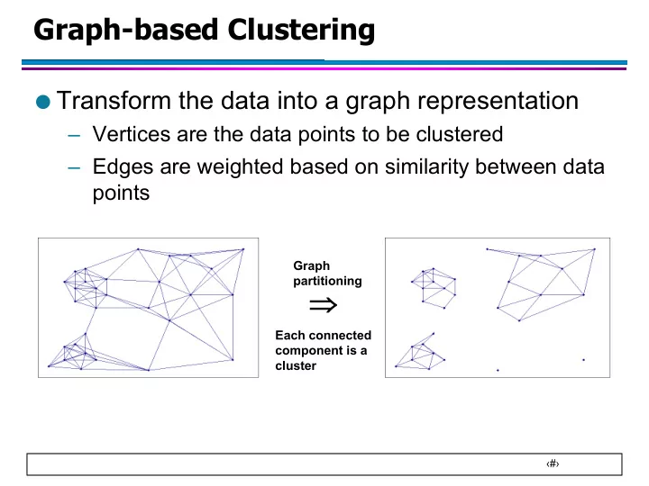
Graph-based Clustering ● Transform the data into a graph representation – Vertices are the data points to be clustered – Edges are weighted based on similarity between data points Graph partitioning Þ Each connected component is a cluster ‹#›

Clustering as Graph Partitioning ● Two things needed: 1. An objective function to determine what would be the best way to “cut” the edges of a graph 2. An algorithm to find the optimal partition (optimal according to the objective function) ‹#›

Objective Function for Partitioning ● Suppose we want to partition the set of vertices V into two sets: V 1 and V 2 – One possible objective function is to minimize graph cut å = Cut ( V , V ) w w ij is weight of the edge between nodes i and j 1 2 ij Î i V 1 , Î j V v 1 v 5 2 v 1 v 5 0.1 0.1 0.1 0.1 0.2 0.2 v 3 v 4 v 3 v 4 0.1 0.3 0.1 0.3 v 2 v 6 v 2 v 6 Cut = 0.2 Cut = 0.4 ‹#›

Objective Function for Partitioning ● Limitation of minimizing graph cut: v 1 v 5 0.1 0.1 0.2 Cut = 0.1 v 3 v 4 0.1 0.3 v 2 v 6 – The optimal solution might be to split up a single node from the rest of the graph! Not a desirable solution ‹#›

Objective Function for Partitioning ● We should not only minimize the graph cut; but also look for “balanced” clusters Cut( V , V ) Cut( V , V ) = + Ratio cut ( V , V ) 1 2 1 2 1 2 | V | | V | 1 2 Cut( V , V ) Cut( V , V ) = + Normalized cut ( V , V ) 1 2 1 2 å å 1 2 d d i j Î Î i V j V 1 2 å = wher e d w i ij j V 2 V 1 V 1 and V 2 are the set of nodes in partitions 1 and 2 |V i | is the number of nodes in partition V i ‹#›

Example v 1 v 5 v 1 v 5 0.1 0.1 0.1 0.1 0.2 0.2 v 3 v 3 v 4 v 4 0.1 0.1 0.3 0.3 v 2 v 6 v 2 v 6 Cut = 0.2 Cut = 0.1 Ratio cut = 0.2/3 + 0.2/3 = 0.13 Ratio cut = 0.1/1 + 0.1/5 = 0.12 Normalized cut = 0.2/1 + 0.2/0.6 Normalized cut = 0.1/0.1 + 0.1/1.5 = 0.53 = 1.07 ‹#›

Example If graph is unweighted (or has the same edge weight) v 1 v 5 v 1 v 5 1 1 1 1 1 1 v 3 v 3 v 4 v 4 1 1 1 1 v 2 v 6 v 2 v 6 Cut = 2 Cut = 1 Ratio cut = 1/3 + 1/3 = 0.67 Ratio cut = 1/1 + 1/5 = 1.2 Normalized cut = 1/5 + 1/5 Normalized cut = 1/1 + 1/9 = 0.2 = 1.11 ‹#›

Algorithm for Graph Partitioning ● How to minimize the objective function? – We can use a heuristic (greedy) approach to do this u Example: METIS graph partitioning http://www.cs.umn.edu/~metis – An elegant way to optimize the function is by using ideas from spectral graph theory u This leads to a class of algorithms known as spectral clustering ‹#›

Spectral Clustering ● Spectral properties of a graph – Spectral properties: eigenvalues/eigenvectors of the adjacency matrix can be used to represent a graph ● There exists a relationship between spectral properties of a graph and the graph partitioning problem ‹#›

Spectral Properties of a Graph ● Start with a similarity/adjacency matrix, W, of a graph ● Define a diagonal matrix D ì n = å ï = w if i j D í ik ij = k 1 ï 0 otherwise î – If W is a binary 0/1 matrix, then D ii represents the degree of node i ‹#›

Preliminaries é ù v 1 v 5 0 0 1 0 0 0 ê ú 0 0 1 0 0 0 ê ú 1 1 ê ú 1 1 0 0 0 0 v 3 Two block- v 4 = W ê ú diagonal matrices 0 0 0 0 1 1 ê ú 1 1 ê ú 0 0 0 1 0 0 ê ú v 2 v 6 ê ú 0 0 0 1 0 0 ë û é ù 1 0 0 0 0 0 Two clusters ê ú 0 1 0 0 0 0 ê ú ê ú 0 0 2 0 0 0 ì n = å = D ê ú ï = w if i j 0 0 0 2 0 0 D ê ú í ik ij = k 1 ê ú ï 0 0 0 0 1 0 0 otherwise î ê ú ê ú 0 0 0 0 0 1 ë û ‹#›

Graph Laplacian Matrix é ù v 1 v 5 0 0 1 0 0 0 ê ú 0 0 1 0 0 0 ê ú 1 1 ê ú 1 1 0 0 0 0 v 3 Two block v 4 = W ê ú matrices 0 0 0 0 1 1 ê ú 1 1 ê ú 0 0 0 1 0 0 ê ú v 2 v 6 ê ú 0 0 0 1 0 0 ë û - é ù 1 0 1 0 0 0 = - Laplacian, L D W ê ú - 0 1 1 0 0 0 ê ú ê ú - - 1 1 2 0 0 0 = L ê ú - - Laplacian also 0 0 0 2 1 1 ê ú has a block ê ú - structure 0 0 0 1 1 0 ê ú - ê ú 0 0 0 1 0 1 ë û ‹#›

Properties of Graph Laplacian ● L = (D – W) is a symmetric matrix ● L is a positive semi-definite matrix – Consequence: all eigenvalues of L are ³ 0 ‹#›

Spectral Clustering Consider a data set with N data points Construct an N ´ N similarity matrix, W 1. Compute the N ´ N Laplacian matrix, L = D – W 2. Compute the k “smallest” eigenvectors of L 3. a) Each eigenvector v i is an N ´ 1 column vector b) Create a matrix V containing eigenvectors v 1 , v 2 , .., v k as columns (you may exclude the first eigenvector) Cluster the rows in V using k-means or other 4. clustering algorithms into K clusters ‹#›

Example ‹#›

Summary ● Spectral properties of a graph (i.e., eigenvalues and eigenvectors) contain information about clustering structure ● To find k clusters, apply k-means or other algorithms to the first k eigenvectors of the graph Laplacian matrix ‹#›

Minimum Spanning Tree ● Given the MST of data points, remove the longest edge (inconsistent) and then the next longest edge,....... ‹#›

‹#›

● One useful statistics that can be estimated from the MST is the edge length distribution ● For instance, in the case of 2 dense clusters immersed in a sparse set of points ‹#›

Cluster Validity l Which clustering method is appropriate for a particular data set? l How does one determine whether the results of a clustering method truly characterize data? l How do you know when you have a good set of clusters? l Is it unusual to find a cluster as compact and isolated as the observed clusters? l How to guard against elaborate interpretation of randomly distributed data? ‹#›

Cluster Validity ● Clustering algorithms find clusters, even if there are no natural clusters in data to design new methods, difficult to validate K-Means; K=3 100 2D uniform data points • Cluster stability : Perturb data by bootstrapping. How do clusters change over the ensemble ‹#› 21 21

Hierarchical Clustering • Hierarchical clustering is a method of cluster analysis which seeks to build a hierarchy of clusters. Two approaches: • Agglomerative ("bottom up“): each point starts in its own cluster, and pairs of clusters are merged as one moves up the hierarchy; more popular • Divisive ("top down“): all points start in one cluster, and splits are performed recursively as one moves down the hierarchy How to define similarity between two clusters or a point and a cluster? ‹#›

Agglomerative Clustering Example • Cluster six elements {a}, {b}, {c}, {d}, {e} and {f} in 2D; use Euclidean distance as a similarity • Build the hierarchy from the individual elements by progressively merging clusters • Which elements to merge in a cluster? Usually, merge the two closest elements, according to the chosen distance ‹#›

Single-link v. Complete-link Hierarchical Clustering Suppose we have merged the two closest elements b and c to obtain clusters { a }, { b , c }, { d }, { e } and { f } To merge them further, we need to take the distance between {a} and {b c}. Two common ways to define distance between two clusters: • The maximum distance between elements of each cluster (also called complete-linkage clustering): max { d ( x , y ) : x ∈ A , y ∈ B } • The minimum distance between elements of each cluster (single-linkage clustering): min { d ( x , y ) : x ∈ A , y ∈ B } Stop clustering either when the clusters are too far apart to be merged or when there is a sufficiently small number of clusters ‹#›

2D PCA Project ction of Iris Data

Mi Mini nimum um S Spa panni nning ng T Tree C Clus usteri ring ng o of 2D PCA Project ction of Iris Data

K-Mea Means s Clusteri ering of Iri Iris s Data (C (Clu lusterin ing A Assig ignment s t shown o on 2 2D P PCA P Proje jectio tion) )

Si Singl gle-lin link Clu lusterin ing of of Iris is Data

Co Comp mplete-lin link Clu lusterin ing of of Iris is Data

Angkor Wat Hindu temple built by a Khmer king ~1,150AD; Khmer kingdom declined in the 15th century; French explorers discovered the hidden ruins in late 1800’s ‹#›

Apsaras of Angkor Wat • Angkor Wat contains the most unique gallery of ~2,000 women depicted by detailed full body portraits • What facial types are represented in these portraits? ‹#›

Clustering of Apsara Faces Single Link 127 facial landmarks 127 landmarks 10 1 2 3 6 4 9 5 7 8 Single Link clusters How to validate the clusters or groups? Shape alignment ‹#›

Ground Truth ‹#› Khmer Dance and Cultural Center

Exploratory Data Analysis 2D MDS Projection of the Similarity matrix Clustering with large weights assigned to chin and nose Example devata faces from the clusters differ largely in chin and nose, thereby reflecting the weights chosen for similarity ‹#›

Exploratory Data Analysis 3D MDS Projection of the Similarity matrix ‹#›

‹#›