
SLIDE 1
1
Geometric Methods for Modelling and Control of Shape-Actuated Underwater Vehicles
Kristi A. Morgansen
Department of Aeronautics and Astronautics University of Washington
2
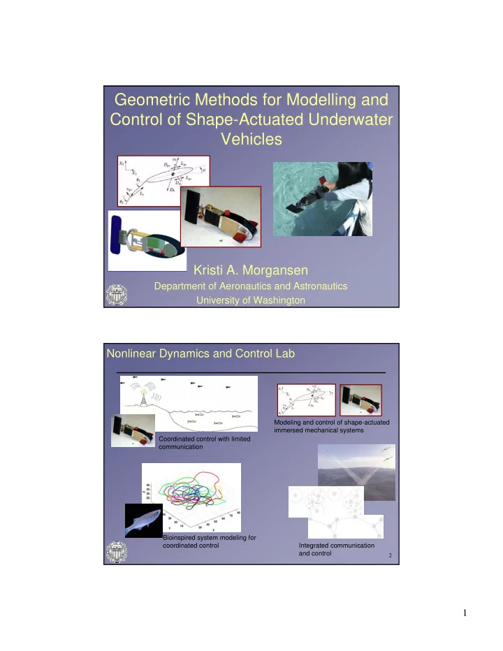
Nonlinear Dynamics and Control Lab
Coordinated control with limited communication Bioinspired system modeling for coordinated control Integrated communication and control Modeling and control of shape-actuated immersed mechanical systems