Formal Verification by Model Checking Jonathan Aldrich Carnegie - PDF document

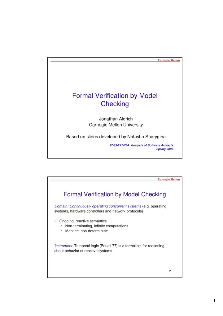
Formal Verification by Model Checking Jonathan Aldrich Carnegie Mellon University Based on slides developed by Natasha Sharygina 17-654/17-754: Analysis of Software Artifacts Spring 2006 1 Formal Verification by Model Checking Domain: Continuously operating concurrent systems (e.g. operating systems, hardware controllers and network protocols) • Ongoing, reactive semantics • Non-terminating, infinite computations • Manifest non-determinism Instrument: Temporal logic [Pnueli 77] is a formalism for reasoning about behavior of reactive systems 2 1

Temporal Logic Model Checking [Clarke,Emerson 81][Queille,Sifakis 82] • Systems are modeled by finite state machines • Properties are written in propositional temporal logic • Verification procedure is an exhaustive search of the state space of the design • Diagnostic counterexamples 3 Temporal Logic Model Checking Finite State Machine Preprocessor Property Model Checker True or Counterexample 4 2

What is Model Checking? Does model M satisfy a property P ? (written M |= P) What is “M”? What is “P”? What is “satisfy”? 5 What is “M”? States: valuations to all variables a b Initial states: subset of states Arcs: transitions between states Atomic Propositions: b c c e.g. x = 5, y = true State Transition Graph or Kripke Model 6 3

What is “M”? M = 〈 S , S 0 , R , L 〉 Kripke structure: S – finite set of states S 0 ⊆ S – set of initial states R ⊆ S × S – set of arcs L : S → 2 AP – mapping from states to a set of atomic propositions 7 Model of Computation a b a b b c c a b c c b c c State Transition Graph Infinite Computation Tree Unwind State Graph to obtain Infinite Tree. A trace is an infinite sequence of states. 8 4

Semantics a b a b b c c a b c c b c c State Transition Graph Infinite Computation Tree The semantics of a FSM is a set of traces . Semantics of the composition of FSMs is the intersection of traces of individual FSMs. 9 What is “P”? Different kinds of temporal logics Syntax: What are the formulas in the logic? Semantics: What does it mean for model M to satisfy formula P ? Formulas: - Atomic propositions: properties of states - Temporal Logic Specifications: properties of traces. 10 5

Computation Tree Logics Examples: Safety (mutual exclusion): no two processes can be at a critical section at the same time Liveness (absence of starvation): every request will be eventually granted Temporal logics differ according to how they handle branching in the underlying computation tree. In a linear temporal logic (LTL), operators are provided for describing system behavior along a single computation path. In a branching-time logic (CTL), the temporal operators quantify over the paths that are possible from a given state. 11 Computation Tree Logics Formulas are constructed from path quantifiers and temporal operators: 1. Path Quantifiers: • A – ‘’for every path’’ • E – ‘’there exists a path’’ 2. Temporal Operator: X α α α - α α α α α holds next time • F α α - α α α α α α holds sometime in the future • α - α G α α α α holds globally in the future α α • α U β - α α α α α α α holds until β holds • 12 6

The Logic LTL Linear Time Logic (LTL) [Pnueli 77]: logic of temporal sequences. Has form A f where f is a path formula which has no path quantifiers ( A or E ) α : α • α α α α α holds in the current state α α α α α α : α • AX α α α α α α holds in the next state α α α α γ : γ • AF γ γ γ γ γ γ holds eventually γ γ γ γ • AG λ λ : λ λ holds from now on λ λ λ λ λ λ λ λ λ λ λ λ λ λ λ λ λ λ λ λ • A ( α α α U β α β β ) : α β α α holds until β α β holds β β α α α α α α α α β β β β 13 The Logic CTL In a branching-time logic (CTL), the temporal operators quantify over the paths that are possible from a given state (s 0 ). Requires each temporal operator ( X , F , G , and U ) to be preceded by a path quantifier ( A or E ). c c c c c c c c c M, s 0 ⊨ AF c M, s 0 ⊨ AG c c c c c M, s 0 ⊨ EF c M, s 0 ⊨ EG c 14 7

Typical CTL Formulas EF ( Started ∧ ¬ ����� ������������������������������������������ �������� ���������� • ������ �������������� AG � ��� ⇒ AF ��� ������������ ��������� ������������������������������ � ������������� � AG � �����!������ ��� DeviceEnabled always holds on every computation path. • AG ( EF Restart ): from any state it is possible to get to the Restart state. 15 Trivia • AG ( EF p ) cannot be expressed in LTL – Reset property: from every state it is possible to get to p a • But there might be paths where you never get to p – Different from A ( GF p ) • Along each possible path, for each state in the path, there b p is a future state where p holds • Counterexample: ababab… 16 8

Trivia • A ( FG p ) cannot be expressed in CTL – Along all paths, one eventually s 0 reaches a point where p p always holds from then on • But at some points in some paths where p always holds, there might be a diverging s 1 s 2 path where p does not hold b p – Different from AF(AG p ) • Along each possible path there exists a state such that p always holds from then on • Counterexample: the path that stays in s 0 17 LTL Conventions • Often leave the initial A implicit • G is sometimes written ⎕ • F is sometimes written ♢ 18 9

Linear vs. branching-time logics some advantages of LTL some advantages of BT logics • LTL properties are preserved • BT allows expression of some under “abstraction”: i.e., if M useful properties like ‘reset’. “approximates” a more complex • CTL, a limited fragment of the model M ’, by introducing more more complete BT logic CTL*, paths, then can be model checked in time M� � ψ ⇒ M ’ � ψ linear in the formula size (as well as in the transition system). • “counterexamples” for LTL are But formulas are usually far simpler: consisting of single executions (rather than trees). smaller than system models, so this isn’t as important as it may • The automata-theoretic approach first seem. to LTL model checking is simpler Some BT logics, like µ -calculus • (no tree automata involved). and CTL, are well-suited for the • anecdotally, it seems most kind of fixed-point computation properties people are interested in scheme used in symbolic model are linear-time properties. checking. 19 Formulas over States and Paths • State formulas – Describe a property of a state in a model M – If p ∈ AP , then p is a state formula – If f and g are state formulas, then ¬ f , f ∧ g and f ∨ g are state formulas – If f is a path formula, then E f and A f are state formulas • Path formulas – Describe a property of an infinite path through a model M – If f is a state formula, then f is also a path formula – If f and g are path formulas, then ¬ f , f ∧ g , f ∨ g , X f , F f , G f , and f U g are path formulas 20 10

Notation • A path π in M is an infinite sequence of states s 0 , s 1 ,… such that for every i ≥ 0, ( s i , s i+1 ) ∈ R • π i denotes the suffix of π starting at s i • If f is a state formula, M , s ⊨ f means that f holds at state s in the Kripke structure M • If f is a path formula, M , π ⊨ f means that f holds along path π in the Kripke structure M 21 Semantics of Formulas M , s ⊨ p ⇔ p ∈ L ( s ) M , π ⊨ f ⇔ π = s… ∧ M , s ⊨ f M , s ⊨ ¬ f ⇔ M , s ⊭ f M , π ⊨ ¬ g ⇔ M , π ⊭ g M , s ⊨ f 1 ∧ f 2 ⇔ M , s ⊨ f 1 ∧ M , s ⊨ f 2 M , π ⊨ g 1 ∧ g 2 ⇔ M , π ⊨ g 1 ∧ M , π ⊨ g 2 M , s ⊨ f 1 ∨ f 2 ⇔ M , s ⊨ f 1 ∨ M , s ⊨ f 2 M , π ⊨ g 1 ∨ g 2 ⇔ M , π ⊨ g 1 ∨ M , π ⊨ g 2 ⇔ M , π 1 ⊨ g M , s ⊨ E g 1 ⇔ ∃ π = s… | M , π ⊨ g 1 M , π ⊨ X g ⇔ ∃ k ≥ 0 | M , π k ⊨ g M , s ⊨ A g 1 ⇔ ∀ π = s… M , π ⊨ g 1 M , π ⊨ F g ⇔ ∀ k ≥ 0 | M , π k ⊨ g M , π ⊨ G g ⇔ ∃ k ≥ 0 | M , π k ⊨ g 2 M , π ⊨ g 1 U g 2 ∧ ∀ 0 ≤ j<k M , π j ⊨ g 1 22 11