FIC graphs Goal: estimate cerebral pathways between brain regions - - PowerPoint PPT Presentation

Graph estimation and selection strategies using the focused information criterion Eugen Pircalabelu

Joint work with Gerda Claeskens, L. Waldorp and S. Jahfari ORSTAT and Leuven Statistic Research Center FICology Workshop, Oslo, May 9-11th, 2016

1 / 24

FIC graphs

Goal: estimate cerebral pathways between brain regions (ROIs) Motivation: ROIs ‘collaborate’/connect to other ROIs: functional connectivity estimate and summarize the structure of the brain graphs targeted FIC approach to focus on parts of the brain How: Framework with both directed & undirected edges Lagged & contemporaneous ROI effects Penalized nodewise models with graph ‘composition’ rules Main contribution: select targeted (via the focus) graphs that account for ROI effects general framework where nodes can be other entities, not just brain ROIs

2 / 24

Motivation

fMRI data: 8 subjects in a resting state study i.e. subjects are not performing any task; parcellation of the brain was obtained containing 68 (further split to 448) regions of interest (ROIs); for each region, 240 volumes of the BOLD signal were obtained;

3 / 24

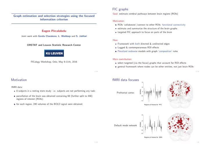
fMRI data focuses

Prefrontal cortex

SIGNAL

−75 −35 35 75

Regions of Interest for PFC

Default mode network

SIGNAL

−50 −25 45 90

Regions of Interest for DMN

4 / 24

Prefrontal cortex focused graph

5 / 24

Graph theoretical framework

Define the graph G = (E, V ) based on edges E nodes V r.v Xi : i ∈ V . To each X1 . . . Xp a node in V = {1 . . . p} is associated. E a subset of V × V set of pairs of distinct nodes. (i, j) ∈ E i → j i parent of j (j, i) ∈ E j → i i child of j (j, i) ∪ (i, j) ∈ E i − j i neighbor of j One or more connections between i and j (directed/undirected); Self-loop edges are allowed (such as i → i) and denote a lagged effect.

6 / 24

Graph selection procedures

1

Graphical Lasso: undirected edges max

Σ−1≻0(log det Σ−1 − tr(W Σ−1) − λ || Σ−1 ||1)

Xi ⊥ Xj|X{1,...,p}\{i,j} iff (i, j) ∪ (j, i) / ∈ E ≡ Σ−1

ij

= 0

2

Neighborhood selection: undirected edges Xi ⊥ Xk|Xnei ∀i ∈ V & ∀k ∈ V \ {nei ∪ i} Xi ‘response node’, other Xj (j = i) covariates in a linear regression. Lasso reg. to determine the neighborhood of node i ˆ neλ

i

= {j ∈ V : ˆ θi

j = 0}

ˆ E λ,AND = {(i, j) : i ∈ ˆ neλ

j AND j ∈ ˆ

neλ

i }

ˆ E λ,OR = {(i, j) : i ∈ ˆ neλ

j OR j ∈ ˆ

neλ

i }

3

Time Series Chain Graphical Models (TSCGM): undirected+directed edges Xt|Xt−1 ∼ N(ΓXt−1, Σ).

7 / 24

Proposed method

the ‘best graph’ should depend on the focus for different focuses, possibly different selected models the focus guides the graph selection aspect Gaussian AR model; penalized nodewise neighborhood selection; mean squared error (MSE) to decide on the selection; Let Y ≡ Xi : i ∈ V the node of interest. W ≡ set of protected nodes, always included as neighbors of Y Z ≡ set of unprotected nodes, potential neighbors Subset S ⊆ V \ i of possible neighbors is to be selected.

8 / 24

Local misspecification

Yk has density f (yk|wk, zk, θ0, γ0 + δ/√n) for k = 1, . . . , n f is 2 times diff. in a ‘proximity’ of (θ0, γ0) (θ0, γ0 + δ/√n) δ controls the proximity around narrow model wk protected neighbors ⇒ θ is present in all models (never subject to model selection or exclusion) (ˆ θ, ˆ γ) = arg max

θ,γ

• 1

n

n

• k=1

log f (yk|wk, zk, θ, γ) − λ n

dγ

• j=1

ψ(|γj − γj0|)

• ,

for a given penalty function ψ (2 times diff. in 0) and an external value λ.

9 / 24

Penalty function

Penalty needed for parameter estimation in p > n settings. FIC takes care of selection so sparse penalties are not necessary. Local quadratic approximation to ψ when not differentiable at zero. lasso : ψl(|γj − γj0|) = |γj − γj0| adaptive lasso : ψal(|γj − γj0|) = wj|γj − γj0|, for a weight wj bridge : ψb(|γj − γj0|) = |γj − γj0|α α > 0 hard thresholding : ψh(|γj − γj0|) = λ2 − (|γj − γj0| − λ)2I(|γj − γj0| < λ) SCAD : ψ

′

s(|γj − γj0|) = I(|γj − γj0| ≤ λ)+

(aλ − |γj − γj0|)+ (a − 1)λ I(|γj − γj0| > λ); a > 2. ψ(|γj − γj0|) ≈ ψ(γjapx) + 1 2 ψ

′(|γjapx|)

|γjapx|

• (γj − γj0)2 − γ2

japx

• ψ(|γj − γj0|)

′ ≈ ψ ′(|γjapx|)

|γjapx| (γj − γj0) ψ(|γj − γj0|)

′′ ≈ ψ ′(|γjapx|)

|γjapx|

10 / 24

Selecting λ

minc

• ωT{J11,S,0ccT(J11,S,0)t − 2(I − GS)δcT(J11,S,0)T}ω
• λS = ωT(I − GS)δ1qT(J11,S,0)Tω

ωTJ11,S,01q1qT(J11,S,0)Tω √n ψ′′(0). Endogeneity problem: MSE ≻ c ≻ λ ≻ (θ, γ) ≻ λ Two-step solution: estim. (θ, γ) on a λ grid, retain (ˆ θ, ˆ γ) with best GCV performance, estimate c and based on c estimate MSE

11 / 24

Focus parameters

Define a focus parameter µ = µ(θ, γ, w, z) a function of θ and γ. µ(σ, β, w, z) = [w, z]tβ; mean of a ROI for fixed vals of other ROIs Eg: For ROI 1

k we define the focus, as the conditional mean on covariates

z = (ROI 2

k , ROI 3 k , ROI 4 k , ROI 1 k−1, ROI 2 k−1, ROI 3 k−1, ROI 4 k−1) as

µ= E[ROI 1

k |z = (−20, 100, 25, 45, 80, 10, 50)]

µ(σ, β, w, z) = βl; reg.coef of a certain ROIl µ(σ, β, w, z) = G −1(0.9|w, z); 0.90-quantile of the response distribution at fixed vals for other ROIs. Goal: estimate µ as precisely as possible (in the MSE sense).

12 / 24

Limiting distribution

For any model S, we compute √n(ˆ µS − µtrue)

d

→ ΛS ∼ N(Bias(µ, S, δ, c), Var(µ, S)), MSE(ˆ µS) = Bias(µ, S, δ, c)2 + Var(µ, S). FIC(G(ES, V )) =

p

• l=1
• MSE(ˆ

µl;Sl), where S = {S1, . . . , Sp|S1 ⊆ {V \ 1}; . . . ; Sp ⊆ {V \ p}}. The mean depends on the chosen focus µ, the submodel S, the value of δ indicating the distance between the parameters from the simplest model and the true model, and on the chosen penalization via the value c = λψ

′′(0)1q/√n. 13 / 24

Graph composition rules

Once all nodewise models are selected (some might include only contemporaneous

• r only dynamic effects, while others might contain both) we apply the ‘OR’ rule

ˆ E λ,or

i−j

=

• (i, j) ∪ (j, i) : ik ∈ ˆ

neλ

jk or jk ∈ ˆ

neλ

ik

• instantaneous undirected

ˆ E λ,or

i→j

=

• (i, j) : ik−1 ∈ ˆ

neλ

jk

• lag 1 directed

ˆ E λ,or

i←j

=

• (j, i) : jk−1 ∈ ˆ

neλ

ik

• lag 1 directed

ˆ E λ,or =

• ˆ

E λ,or

i−j

∪ ˆ E λ,or

i→j ∪ ˆ

E λ,or

i←j

• directed and undirected

where ˆ neλ denotes the neighborhood of the considered node for a certain value of the penalty.

14 / 24

Prefrontal cortex and Default mode network as focuses

Focus FIC LQA ℓ1 FIC ℓ2

15 / 24

Ratio vs FIC GL-CV(Lik) GL-StARS MSPE (PFC focus) 1.52 1.11 MSPE (DMN focus) 1.44 1.06

• No. of edges (PFC focus)

4.67 10.3

• No. of edges (DMN focus)

4.40 9.70

Table: Ratios of the empirical MSPE and number of edges in the estimated graphs for GL-CV(Lik) and GL-StARS relative to the graphs estimated using FIC - LQA ℓ1 for the PFC and DMN focuses.

16 / 24

Small-worldness

1 120 240 0.5 0.8 1.1 Sub.1 Sub.2 Sub.3 Sub.4 Sub.5 Sub.6 Sub.7 Sub.8

Figure: Example of a ‘small-world’ network (left panel) and smoothed ‘small-world’ index (right panel) computed for networks estimated at each time point, for eight subjects.

17 / 24

An average model

FIC LQA ℓ1 GL-StARS

18 / 24

Synthetic data

Multivariate data generated from 3 different graph structures; Independent or time-dependent observations; n ∈ {15, 30, 75, 150, 300}; p ∈ {35, 150}; Constant or non-constant variance over the nodes; Focuses for FIC:

µ1 = µ(θ, γ; ˜ x) evaluated at the ˜ x values corresponding to Huber’s robust location

• f the center of the distribution;

µ2 = µ(θ, γ; ˜ x) evaluated at the ˜ x values that correspond to the median values of the measurements of each node.

˜ x either in-/out-of-sample evaluation point

NODE NODE NODE

• 19 / 24

In;Ct In;Non-ct Out;Ct Out;Non-ct µ2 µ2 µ2 µ2 FIC - ℓ2 0.07 0.13 0.07 0.13 FIC - LQA SCAD 0.07 0.13 0.07 0.13 TSCGM (eBIC) 0.13 0.23 0.14 0.25 TSCGM (BIC) 0.13 0.24 0.15 0.27 TSCGM (GIC) 0.13 0.24 0.14 0.27

Table: Empirical MSPE of estimated graphs for µ2, pooled across 300 simulation runs and 24 different simulation settings. ‘In/Out’ refer to the settings where the point was an in/out-sample,‘Ct/Non-Ct’ refer to settings where the variance at each node was constant or non-constant (randomly sampled at each node).

20 / 24

In;Ct In;Non-ct Out;Ct Out;Non-ct µ2 µ2 µ2 µ2 FIC - ℓ2 0.012 0.025 0.024 0.051 FIC - LQA ℓ1 0.014 0.026 0.035 0.081 GL (CV-Likelihood) 0.035 0.082 0.032 0.075 GL (CV-Trace) 0.041 0.089 0.040 0.081 GL (StARS) 0.041 0.087 0.037 0.079 GL (eBIC) 0.049 0.090 0.047 0.082 CLIME (StARS) 0.051 0.087 0.049 0.079 CLIME (CV-Likelihood) 0.046 0.086 0.043 0.078 CLIME (CV-Trace) 0.048 0.087 0.045 0.079 TIGER (StARS) 0.040 0.087 0.037 0.079 TIGER (CV-Likelihood) 0.048 0.088 0.046 0.080

Table: Empirical MSPE of estimated graphs for µ2, pooled across 300 simulation runs and 60 different simulation settings. ‘In/Out’ refer to the settings where the point was an in/out-sample, ‘Ct/Non-Ct’ refer to settings where the variance at each node was constant or non-constant (randomly sampled at each node).

21 / 24

In;Ct In;Non-ct Out;Ct Out;Non-ct µ2 µ2 µ2 µ2 FIC - ℓ2 0.94 0.92 0.94 0.93 FIC - LQA ℓ1 0.90 0.90 0.89 0.88 GL (CV-Likelihood) 0.69 0.85 0.71 0.87 GL (CV-Trace) 0.78 0.99 0.82 1.00 GL (StARS) 0.90 0.95 0.89 0.94 GL (eBIC) 0.96 1.00 0.96 1.00 CLIME (StARS) 0.97 0.96 0.97 0.96 CLIME (CV-Likelihood) 0.77 0.54 0.77 0.55 CLIME (CV-Trace) 0.83 0.75 0.83 0.74 TIGER (StARS) 0.94 0.96 0.94 0.96 TIGER (CV-Likelihood) 0.97 0.96 0.97 0.96

Table: Sparsity index of estimated graphs for µ2, pooled across 300 simulation runs and 60 different simulation settings. ‘In/Out’ refer to the settings where the point was an in/out-sample, ‘Ct/Non-Ct’ refer to settings where the variance at each node was constant or non-constant (randomly sampled at each node).

22 / 24

Extensions

combined-data model: pooling information from all 8 subjects while allowing for subject specific effects; penalized high-dim. nodewise GLM social network models: what if the graph is given? i.e. a link shows who sends messages to whom. Focuses pertain to parameters of Exponential Random Graph Models (ERGMs), network auto-correlation models and centralization measures.

23 / 24

Take home message

• Our procedures extend the FIC use to select graphical models;
• Selected graphs are targeted to a particular focus for which the estimator

should have a low MSE;

• FIC graph construction useful to estimate brain networks with small MSE;
• Comes closer to the goals of personalized medicine;

24 / 24