Evaluation of Data Needs to Support Water Quality Models for - - PDF document

4/2/2019 1

Evaluation of Data Needs to Support Water Quality Models for Setting Nutrient Targets

Tuesday, April 2, 2019 12:00 – 2:00 pm ET

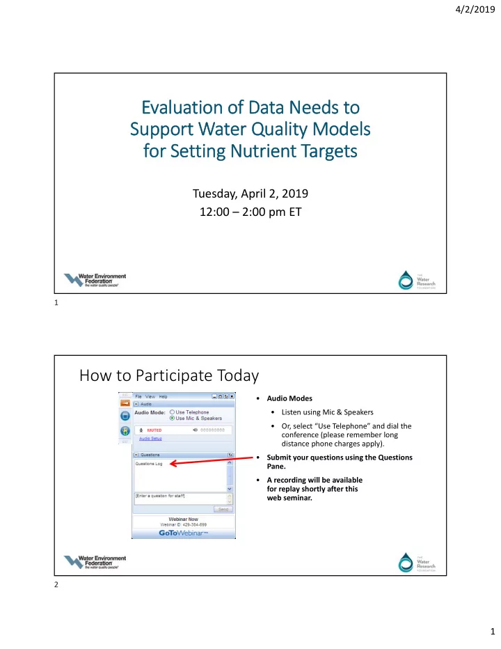
How to Participate Today

• Audio Modes
• Listen using Mic & Speakers
• Or, select “Use Telephone” and dial the

conference (please remember long distance phone charges apply).

• Submit your questions using the Questions

Pane.

• A recording will be available

for replay shortly after this web seminar. 1 2

4/2/2019 2

Today’s Moderators

Lola Olabode Program Director The Water Research Foundation Penelope Moskus Senior Environmental Scientist/Project Manager LimnoTech

Agenda

12:00 Welcome and Introduction 12:10 Rationale for the Project/Steve Chapra 12:20 Project Overview/Todd Redder 12:25 Review of Existing Model Applications/Todd Redder 12:35 Relationship between Amount of Data and Model Utility/Dave Dilks 12:50 Practical Methods for Assessing Model Uncertainty/Dave Dilks 1:15 Requirements for Regulatory Acceptance/Dave Dilks 1:30 Summary of Findings and Project Benefits/Steve Chapra 1:40 Q&A 2:00 Closing

3 4

4/2/2019 3

Today’s Speakers

Steve Chapra, Ph.D. Professor, Civil and Environmental Engineering Tufts University David W. Dilks, Ph.D. Vice President LimnoTech Todd Redder, PE Environmental/Water Resources Engineer LimnoTech

Acknowledgments

• Association of Clean Water Administrators – Special webcasts
• Water Environment Federation – Education and Training
• ACWA‐WEF partnership‐ Permit Writers Workshops
• National Association of Clean Water Agencies –Committee updates, Briefings, Support to the Utilities
• Colorado Monitoring Framework – Reg 85, Colorado Water Quality Control Commission
• EPA – Briefings, Information Exchange and Updates
• American Water Resources Association‐ Information Exchange
• The California Water and Environmental Modeling Forum – Information exchange
• Utilities – Participation, Information Exchange, Case Studies, Demonstrations, and Implementation of Water

Quality Based Discharge Standards.

• States – Participation, Information Exchange, Case Studies, Demonstrations, and Implementation of Water

Quality Based Discharge Standards.

• Key Consultants & Academics – (LimnoTech, Brown & Caldwell, Clements consulting, Arcadis, Dr. Steve Chapra)
• WRF’s Sustainable Integrated Water Management and Nutrients Research – Collaboration, Information

Exchange, and Strategic communications

5 6

4/2/2019 4

Enable the water quality community to fully participate in the development and implementation of water quality based discharge standards for contaminants (principally nutrients) by developing independent methods for confirming linkages between receiving water quality, wastewater discharges, and

• ther sources.

Research Area Objective

Research Projects Receiving Water Linkages in Water Quality (LINK)

Year Project Title Research Group

Linkages Permit Comm.

2019

2019 Roadmap on prioritizing research in both permitting and linkages

X X X 2018

Modeling Guidance for Developing Site Specific Nutrient Goals – Demonstration, Screening‐Level Application (LINK4T17).

X X X 2017

Establishing Methods for Numeric Nutrient Target‐Setting (LINK3R16)

X X 2015

Developing Site‐Specific Nutrient Goals – Demonstration: Boulder Creek, Colorado (LINK2T14)

X 2015

Modeling Guidance for Developing Site‐Specific Nutrient Goals (LINK1T11)

X 2010

Linking Receiving Water Impacts to Sources and to Water Quality Management Decisions: Using Nutrients as an Initial Case Study (WERF3C10, 2010)

X

7 8

4/2/2019 5

Rationale for Project

• Nutrient pollution is a serious concern
• The relationship between nutrients and

environmental response is complicated

• Guidance is needed on methods for conducting

rigorous site‐specific assessments to set nutrient targets

Nutrient Pollution is a Serious Concern

• Excess nitrogen and phosphorus is a major

water quality concern

─>10,000 waters impaired nationally ─Harmful algal blooms are increasing

• EPA has been calling for states to develop

numeric nutrient criteria for more than a decade

9 10

4/2/2019 6

Relationships between Nutrients and Endpoints Are Complicated

• Response of aquatic plants to nutrient loads are highly

dependent on site‐specific factors

─e.g., clarity, shading, habitat, hydrology

• Multiple potential endpoints

─e.g., hypoxia, harmful algal blooms, aesthetics

• Many endpoints of concern require consideration of multiple

levels of relationships

─Nutrients ‐> algal growth‐> algal toxins

Methods for Developing Numeric Nutrient Criteria

EPA has defined three categories of approaches

• 1. Reference condition approach
• Base numeric nutrient criteria at levels consistent with those observed in

relatively pristine (i.e. “reference”) water bodies

• 2. Stressor‐response analysis
• Empirically derive statistical relationships between in‐situ nutrient

concentrations and the response variable

• 3. Process‐based (mechanistic) modeling
• Describe systems using equations representing specific ecological processes,

calibrated to site‐specific data

11 12

4/2/2019 7

The Most Readily Applied Approaches Can Be Inaccurate

Reference condition approach can be (relatively) easily applied to broad areas, but is potentially very imprecise

─Doesn’t consider the dose‐response relationship between nutrients and environmental response

• Unable to define the threshold where impairment begins

─Doesn’t consider potentially important site‐specific factors

The Most Readily Applied Approaches Can Be Inaccurate

Stressor‐response analysis considers thresholds, but still not accurate for all sites

─Doesn’t consider important site‐specific factors ─Correlation does not mean causation

Higher TN, but good biology

13 14

4/2/2019 8

Simple Approaches Can Result in Expensive Controls

• Existing TMDLs using reference condition‐based numeric

nutrient criteria have led to some extremely low wasteload allocations to WWTPs for nutrients

─TP = 0.007 mg/l ─TN = 0.289 mg/l

• No assessment of site‐specific response to nutrient levels

conducted

Guidance Is Needed on Rigorous Methods for Nutrient Criteria

• EPA provides guidance for developing nutrient criteria using the

reference condition and stressor‐response approaches

• Similar guidance is not currently available for the process‐based

modeling approach

─Lack of guidance will serve as an impediment for more rigorous approaches being taken

15 16

4/2/2019 9

WRF Predecessor Projects on Rigorous Methods for Nutrient Criteria

• LINK1T11

─Developed a Nutrient Modeling Toolbox/Model Selection Decision Tool to select models for specific sites

• LINK2T14

─Applied Nutrient Modeling Toolbox to Boulder Creek, CO

• Selection of an appropriate model is not enough, also need

sufficient data

Project Overview Project Objectives and Team

17 18

4/2/2019 10

Project Objectives

Overarching: Determine how much data is needed to successfully apply a model to set nutrient targets

• 1. Define relationship between data availability and model utility
• 2. Assess methods for estimating model uncertainty
• 3. Provide insight into the regulatory climate regarding consideration
• f model uncertainty

Project Team

WRF Issue Area Team Stakeholder Advisory Panel

• Lola Olabode, WRF
• Raj Bhattarai, P.E., BCEE,

City of Austin, TX

• Renee Bourdeau, P.E.,

Horsley Witten Group

• Xueqing Gao, Ph.D., FL

Department of Health

• Bret Linenfelser, City of

Boulder

• Steve Peene, Ph.D., ATM
• Jim Pletl, Ph.D., HRSD
• Paul Stacey, Footprints in

the Water, LLC

• Thomas Stiles, KDHE
• Steve Whitlock, PE, EPA
• Matt Wooten, SD No. 1 of

Northern Kentucky

• Tom Fikslin, Ph.D. Retired

River Basin Commission

• Lewis Linker, U.S. EPA

Chesapeake Bay Program Office

• Mindy Scott, Sanitation

District No. 1 of Northern Kentucky

• Elizabeth Moore,

Montgomery County (OH) Environmental Services

Co‐Principal Investigators Project Manager

• David W. Dilks, Ph.D., LimnoTech
• Todd M. Redder, PE, LimnoTech
• Steven C. Chapra, Ph.D., F. ASCE, Tufts University
• Penelope Moskus, LimnoTech

Project Team

• Victor J. Bierman Jr., Ph.D., BCEEM (Senior Advisor)
• Joseph V. DePinto, Ph.D. (Senior Advisor)
• Derek Schlea, PE. LimnoTech
• Daniel Rucinski, Ph.D., LimnoTech
• Hua Tao, Ph.D., LimnoTech
• Scott C. Hinz, LimnoTech
• Kyle Flynn, Ph.D., P.E., P.H.,KF2 Consulting, PLLC
• Nicole Clements, Clements Consulting

19 20

4/2/2019 11

Project Summary Overview of Tasks

Project Tasks

• 1. Review existing models applied to set nutrient targets
• 2. Assess relationship between amount of data and model utility

at data‐rich case study sites

• 3. Develop practical methods for assessing model uncertainty
• 4. Assess requirements for regulatory acceptance

22

21 22

4/2/2019 12

Review of Existing Model Applications

• Gain insight into how much data was required to support

management decisions at other sites

• Develop broad inventory of applications

–At least five examples from rivers, lakes, and estuaries –At least five examples for each key endpoint –At least five examples of applications that were, and were not, successful in defining nutrient targets for regulatory purposes

Inventory of Model Applications

• Gathered 38 nutrient modeling applications

─Diversity of water bodies within various regions ─20 sites with dissolved oxygen, 22 with sestonic chlorophyll, and 7 with attached algae endpoints

Region U.S. EPA Regions Estuary Lake/Impoundment River North Central (MT, WY, UT, CO, ND, SD, NE, KS, IA, MO, MN, WI, IL, IN, MI, OH) 5, 7, 8 ‐‐ 9 4 Northeast (ME, NH, VT, MA, RI, CT, NY, NJ, PA, WV, VA, DE, MD, DC) 1, 2, 3 ‐‐ 1 3 Northwest (AK, ID, OR, WA) 10 1 2 4 South Central (NM, TX, OK, AR, LA) 6 ‐‐ 1 ‐‐ Southeast (KY, TN, MS, AL, GA, FL, NC, SC) 4 8 7 1 Southwest (AZ, CA, HI, NV) 9 1 1 2 Total 10 21 14

23 24

4/2/2019 13

Review of Existing Model Applications

• Characterized each of the model applications regarding the

following features:

─Data availability ─Model calibration evaluation ─Uncertainty assessment ─Regulatory/management outcome

• Fifteen individual assessments made

─Ranked on a 1‐5 scale

Review of Model Applications

High Degree of Rigor: State of the Science Moderate Rigor Low Degree of Rigor: Default Values

5 4 3 2 1

Spatial Captures all of the important spatial variability; required spatial resolution of data explicitly assessed; data available at desired resolution. Captures most of the important spatial variability; required spatial resolution of data given consideration; data available at desired resolution. Captures some of the important spatial variability; spatial variability of data included, with cursory consideration of necessary extent. Some spatial variability included, but no consideration of necessary extent. No spatial variability included; necessary extent not considered. Temporal Resolution Captures all of the important temporal variability; required temporal resolution explicitly assessed; data available at desired resolution. Captures most of the important temporal variability; required temporal resolution assumed; data available at desired resolution. Captures some of the important spatial variability; temporal variability of data included, with less than complete coverage. Some temporal variability exists, many gaps present. No temporal variability included; necessary extent not considered. Temporal Extent Greater than five years (or steady state periods) of data. Three to five years (or steady state periods) of data. Two years (or steady state periods) of data. One year (or steady state period) or less of data. No calibration data available. Parameters Data available for all state variables, except for those demonstrated to be unimportant. Data available for all state variables, except for those presumed to be unimportant. Data available for many state variables, some potentially important parameters absent. Missing most state variables. No calibration data available.

Evaluation Criteria for Data Availability: Model Calibration Data

25 26

4/2/2019 14

Comparison of Successful vs. Unsuccessful Applications

• Question: For which parameters did more rigorous data and/or

approach lead to an accepted model?

• Approach: Statistically compared “rigor” scores between

‘successful’ and ‘unsuccessful’ applications

Successful vs. Unsuccessful Applications

• No significant difference between successful and unsuccessful

applications were found for any of the parameters

27 28

4/2/2019 15

Regulatory Significance Is Important

• Positive correlation found between degree of rigor and

regulatory significance for every factor evaluated.

• Graded approach to model application

1 2 3 4 5 1 2 3 4 5

Spatial Forcings Rigor Regulatory Significance

Example Result:

Finding: Review of Existing Models

• The amount of data required for a model application depends

upon the regulatory significance of the application

1 2 3 4 5 1 2 3 4 5

Data Requirements Regulatory Significance

29 30

4/2/2019 16

Assessment of Relationship between Amount

• f Data and Model Utility
• Evaluate model robustness by

characterizing the uncertainty that results from different levels of data availability

• Examined through Jackknife Assessment
• Conducted for two data‐rich case study

sites

• Truckee River, NV
• Western Basin of Lake Erie

Jackknife Example

• Conduct calibration multiple times, excluding a portion of

the data set each time

• Simple first‐order decay example: C = Coe‐kt

Time Conc. 1 97.9 2 90.9 3 45.5 4 44.6 5 18.7

Data Estimation of Decay Rate

31 32

4/2/2019 17

Jackknife Example

• Exclude first data point, estimate decay rate

Time Conc. 1 97.9 2 90.9 3 45.5 4 44.6 5 18.7

Data Estimation of Decay Rate

Jackknife Example

• Repeat by excluding additional data points
• Compile all results to assess uncertainty in parameter(s)

33 34

4/2/2019 18

Jackknife Case Study Sites

• Truckee R., NV
• HSPF model developed to

assess revision to existing WQS for nitrogen

• Endpoints of concern were

dissolved oxygen, periphyton density

Jackknife Case Study Sites

• Western Basin of Lake Erie
• A2EM model developed to

assess control of harmful algal blooms

• Endpoints of concern were

harmful algal blooms, chlorophyll a

35 36

4/2/2019 19

Combinations Considered during Jackknife Analysis

• 74 combinations of years evaluated for Truckee

─ 6 combinations of five years (leave one out) ─ 15 combinations of four years (leave two out) ─ 20 combinations of three years (leave three out) ─ 15 combinations of two years (leave four out) ─ 6 combinations of one year (leave five out) ─ 12 combinations of half years

• 40 combinations of years evaluated for Lake Erie

─ 5 combinations of four years (leaving one year out) ─ 10 combinations of three years (leave two out) ─ 10 combinations of two years (leave three out) ─ 5 combinations of one year (leave four out) ─ 10 combinations of half years

Processing Jackknife Results

• Evaluated model prediction

error for different parameter combinations and different years

─Maximum benthic algal growth rate ─Benthic algal respiration rate ─Reaeration rate escape coefficient

37 38

4/2/2019 20

Jackknife Findings

• “Apparent accuracy”* of model decreases with additional data

*How well model describes available data

0.40 0.45 0.50 0.55 0.60

1 2 3 4 5

Average Aggregate Error Years of Data

Jackknife Findings

• “Actual model error”* decreases with additional data

*How well model describes all data

39 40

4/2/2019 21

Findings: Case Study Evaluations

• Traditional metrics for model performance

do better with less data

• Rigorous assessment of model

performance indicates more years of data result in lower error

Practical Methods for Assessing Model Uncertainty

• The inability to quantify model uncertainty was

identified as limitation of the models in the Nutrient Management Toolbox

• Reviewed applicability of seven methods via testing
• n real world model applications

Methods That Don’t Consider Observed Data

• Sensitivity analysis
• First order variance analysis

Methods That Do Consider Observed Data

• Generalized sensitivity analysis
• One parameter at a time Bayesian
• Markov Chain Monte Carlo
• Full Bayesian approaches
• Bounding calibration

41 42

4/2/2019 22

Simpler Model Uncertainty Analyses

• Sensitivity analysis, first‐order error analysis

─Pre‐specify uncertainty in input parameters ─Simulate range of model response corresponding to given range in inputs

Simpler Model Uncertainty Analyses

• Do not consider the ability of specified input uncertainty to

describe observed data

• Can give credence to model results that are inconsistent with

real world

43 44

4/2/2019 23

Bayesian Approaches

• Consider the ability of given parameter values to describe
• bserved data

– Quantify goodness of fit with a likelihood function, L

L = 0.01 L = 0.03

Bayesian Approaches

• Can also consider prior

knowledge of parameter uncertainty

─Sample priors using Monte Carlo (or Latin Hypercube)

45 46

4/2/2019 24

Bayesian Approaches

• Resulting matrix can be used to:

─Assess marginal probability distributions

• Construct histograms

using likelihood to weight values

• Examine uncertainty in model predictions
• Run simulation for each parameter set, weight results by likelihood

Generalized Sensitivity Analysis

• Similar to Bayesian approach,

but

─Doesn’t presume shape of prior distributions ─Assesses whether each individual simulation “does” or “does not” adequately describe the data

47 48

4/2/2019 25

Bayesian Model Uncertainty Analyses

• Can have excessive

computational requirements

─Consideration of ten different values for each

• f 100 parameters

would require 10100 (i.e.,

• ne Googol) simulations

Worst Case Bounding Calibration

• Similar to generalized

sensitivity analysis

─Use judgment to find acceptable parameter sets

• Conduct scenario

analysis using parameter set that generates “worst‐case” results

1 1 1

• 1. Select

parameter value

• 2. Perform

simulation

• 3. Evaluate

likelihood as yes/no

• 4. Store

acceptable parameter sets

• 5. Repeat

steps 1‐4

49 50

4/2/2019 26

Markov Chain Monte Carlo

• Bayesian approach with more intelligent

parameter selection

– Use information gained from prior simulations to select values for next simulation – Focuses parameter selection on values more likely to adequately describe

• bserved data

Real World Uncertainty Application

• Applied range of techniques to existing model

applications to assess feasibility

‐ Yellowstone R.

• One‐at‐a‐time Bayesian,

generalized sensitivity analysis, worst case bounding calibration

‐ Fountain Lake

• Markov Chain Monte

Carlo

‐ Truckee R.

• Worst case bounding

calibration, generalized sensitivity analysis

‐ Lake Erie

• Worst case bounding

calibration, generalized sensitivity analysis

51 52

4/2/2019 27

Lake Erie Uncertainty Results

• Conducted 420 calibration runs to define eight

acceptable parameter sets

Growth Rate Half Saturation Organic Settling Rate Blue Green Optimal Growth Temperature +25% +50% Calibration Calibration +25% +50% +50% Calibration +25% Calibration ‐50% Calibration +25% +50% ‐50% Calibration Calibration +50% ‐50% +20% +25% +50% ‐50% +20% +25% Calibration ‐50% +20% +25% +50% Calibration +20%

Lake Erie Uncertainty Results

• Findings

─No single parameter set represents “worst case” for all conditions ─Computational time is a concern

53 54

4/2/2019 28

Yellowstone R. Bounding Calibration/ Generalized Sensitivity Analysis

• 177 different parameter sets were identified that

resulted in an “acceptable” calibration

• Numeric nutrient criterion scenario runs

conducted to evaluate instream pH in response to ten different hypothetical TP concentrations

Yellowstone R. Bounding Calibration/ Generalized Sensitivity Analysis

• 177 results per concentration allows frequency

distributions to be assessed

55 56

4/2/2019 29

Yellowstone R. Findings

• Models with fast execution times are amenable to more

rigorous application of uncertainty techniques

─Generalized sensitivity analysis with more parameters considered or one‐at‐a‐time Bayesian ─Better suited to evaluate Type I and Type II error

Fountain Lake Phytoplankton Model

• Dynamic spreadsheet model developed to assess

management options for controlling algae in a lake receiving wastewater discharge

• Applied Markov Chain Monte Carlo (MCMC)

─Shuffled Complex Evolution Metropolis algorithm was implemented in MATLAB ─Tested resources required for different amounts of uncertain parameters

57 58

4/2/2019 30

Fountain Lake MCMC

• Time to convergence depends upon number of parameters treated

as uncertain

One parameter: 100 iterations Two parameters: 400 iterations Five parameters: 5000 iterations

• Feasibly applied to only to simpler models

Review of Uncertainty Analysis Methods

Advantages Disadvantages Summary Sensitivity Analysis  Simple to apply.  Should be conducted as part of standard modeling practice.  Does not provide useful information on model uncertainty. Insufficient to serve as a stand‐ alone method for uncertainty assessment, but useful for identifying important parameters. First Order Variance Analysis  Manageable computational requirements.  Considers combined effect of multiple uncertain parameters.  Requires prior knowledge of parameter uncertainty.  Assumes linear response between parameter change and model results. Potentially suitable if parameter uncertainty is well characterized and model response to uncertainty is linear. One Parameter at a Time Bayesian  Considers ability of uncertain parameter values to describe

• bserved data.

 Excessive computational requirements for models with long execution times.  Does not consider correlation structure between acceptable input values. Potentially suitable for models with shorter execution times. Bounding Calibration  Considers ability of uncertain parameter values to describe

• bserved data, including

correlation structure.  Lower computational requirements.  “Worst case” parameter set can be difficult to define, and may not exist.  Provides no assessment of Type II errors. Potentially suitable for models where worst case parameter set exists and can be readily identified. Generalized Sensitivity Analysis  Considers ability of uncertain parameter values to describe

• bserved data, including

correlation structure.  Impractical to identify all acceptable parameter combinations.  Decision as to what represents an “acceptable” calibration introduces some subjectivity. Suitable if limited to assessment

• f most important parameters.

Full Bayesian Approaches  Considers ability of uncertain parameter values to describe

• bserved data, including

correlation structure.  Impractical to sample entire range of parameter combinations Potentially suitable for models with limited number of parameters and/or shorter execution times. Markov Chain Monte Carlo  Considers ability of uncertain parameter values to describe

• bserved data.

 More efficient than standard Bayesian approaches.  Requires computer coding to implement.  Impractical computational times for complex models. Best suited for research applications, or models with very short execution times.

59 60

4/2/2019 31

Model Uncertainty Finding #3

• Computationally tractable approaches (sensitivity

analysis, first order variance analysis) provide limited information

• Approaches that consider ability of parameter values

to describe observed data are computationally impractical for highly parameterized models

• “Worst‐case” parameter set varies with environmental

conditions

“Practical” Uncertainty Analysis

• Builds off of typical modeling best

practices

• 1. Conduct model sensitivity analysis
• 2. Define “acceptable” model calibration
• 3. Maintain a model run log during

calibration process

• 4. Supplement acceptable parameter sets as

practical

• 5. Conduct scenario evaluations using all

acceptable parameter sets

61 62

4/2/2019 32

Requirements for Regulatory Acceptance

• “How good does a model need to be (or how much

data is required) for it to be accepted?”

• Addressed in two ways

─Interviewed regulatory staff from six States ─Reviewed common factors for “accepted” model applications in model inventory

Findings on Regulatory Acceptance

• Formal protocols for assessing the quality of modeling are not

applied on a widespread basis

─Steps are being made

• Confounding factors

─Variation in data requirements across endpoints and water body types ─Difficulties in quantifying model uncertainty ─Lack of protocols for incorporating uncertainty in decision making

• Presence of external review panel facilitates model acceptance

63 64

4/2/2019 33

Regulatory Acceptance Recommendations (Pt. 1)

• Consider inclusion of peer review input at project
• utset for potentially contentious situations
• Apply model prior to data collection to assess spatial

and temporal requirements

Regulatory Acceptance Recommendations (Pt. 2)

• Include consideration of uncertainty during decision‐making

to assess likelihood of requiring nutrient targets that are:

─too lenient to protect the designated use ─more stringent than necessary to protect the designated use

65 66

4/2/2019 34

Monitoring Recommendations

Category Data Requirements Model Forcing Functions Spatial Coverage

Monitoring station(s) at upstream boundary (or boundaries, for a branched system). Monitoring station at each tributary or point source that the scoping model indicates will change instream concentration

• f any state variable of concern by more than a predetermined amount (e.g. 1%). If economically feasible, samples

above and below the mixing zone of major inputs should be collected.

Temporal Frequency

Sufficient to capture any important temporal variability in forcing functions:

• If dissolved oxygen is an endpoint of concern, continuous dissolved oxygen and temperature at all boundaries where

the diel signal from the source propagates throughout the model.

• Three to four sampling periods per independent survey event for other forcing functions, unless observed variability

dictates more frequent sampling.

Temporal Extent

Duration of sampling should be longer than time of travel from upstream to downstream boundary.

Sampling Parameters

Loads of all nutrient forms and organic carbon represented as state variables in the selected model framework. Dissolved oxygen, temperature, flow, suspended solids, conductivity.

Ambient Calibration Data Spatial Coverage

Stations located with sufficient resolution to capture any significant (e.g. >10% change) gradient in important state variables as predicted by the scoping model. Stations located no more than 0.5 days travel time apart in absence of spatial gradients. Additional stations located corresponding to any significant resource areas of concern.

Temporal Frequency

Sufficient to capture any important temporal variability in forcing functions:

• Continuous dissolved oxygen and pH, if these are endpoints of concern.
• Three to four sampling periods per independent survey event for other calibration parameters, unless observed

variability dictates more frequent sampling.

Sampling Parameters

Concentrations of all state variables considered by the model.

Number of Events

Minimum of two independent survey events representative of critical (or near critical) environmental conditions.

Key Processes

Sediment oxygen demand, if dissolved oxygen is an endpoint of concern.

• Although “one size

doesn’t fit all”, monitoring recommendations are provided for different water body types

Consideration of Uncertainty

• Use uncertainty analysis results to examine the risks associated

with requiring nutrient targets that are: ─too lenient to protect the designated use ─more stringent than necessary to protect the designated use

• Depending on uncertainty method used, can either examine:

Range of results Probability of each type of error

67 68

4/2/2019 35

Summary of Key Findings

• More data does not translate into improved model

performance*

• Quantity of data necessary to support a model varies widely
• Methods to accurately define uncertainty are not easily applied
• Regulatory requirements for amount of data/model

performance are not clearly defined

*For most commonly used calibration metrics

Project Benefits

• Guidelines developed summarizing data requirements to

support models for different endpoints and water body types

• Practical method proposed for conducting uncertainty

analysis on complex models

• Guidance developed on maximizing likelihood of model

acceptance

69 70

4/2/2019 36

Questions for Our Speakers?

• Submit your questions

using the Questions Pane.

Thank you!

For additional information, contact: Lola Olabode lolabode@waterrf.org

71 72