
SLIDE 1
Estimating with uncertainty
Chapter 4
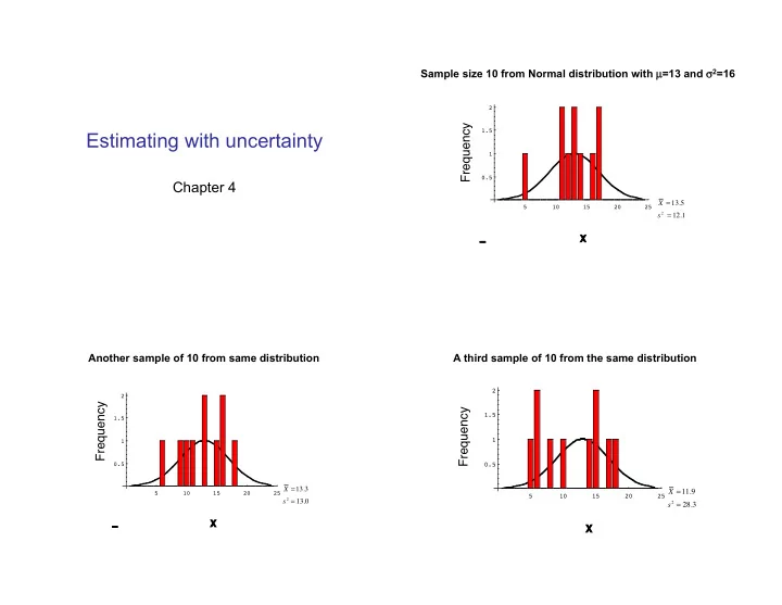
5 10 15 20 25 0.5 1 1.5 2
X = 13.5
s 2 = 12.1
_ X
Sample size 10 from Normal distribution with µ=13 and 2=16
Frequency
Another sample of 10 from same distribution
5 10 15 20 25 0.5 1 1.5 2
X =13.3 s 2 = 13.0
_ X
Frequency
A third sample of 10 from the same distribution
5 10 15 20 25 0.5 1 1.5 2
X =11.9 s 2 = 28.3
X
Frequency