E X p p S d S r ( ) r , - - PDF document

Skewness and Kurtosis Estimation Method for Fission Source Convergence Diagnosis in Monte Carlo Eigenvalue Calculations

Ho Jin Park and Jin Young Cho

aKorea Atomic Energy Research Institute, 111, Daedeok-daero 989beon-gil, Daejeon, 34057, Korea *Corresponding author: parkhj@kaeri.re.kr

• 1. Introduction

In a conventional Monte Carlo (MC) eigenvalue transport calculation, the so-called inactive cycle MC runs are performed to provide stationary

• r

fundamental-mode fission source distribution (FSD). The inactive cycle MC runs need to continue until the current FSD converges to the stationary FSD. Determining the number of inactive cycles is an important concern in obtaining unbiased MC solutions. However, it is difficult for a user of the MC code to recognize whether the number of inactive cycles is sufficiently large. Accordingly, many studies [1,2] for convergence criteria in MC eigenvalue calculations have been conducted to resolve this question. We propose a way in which the skewness and kurtosis [3,4,5] can be used to test for convergence criteria in MC eigenvalue calculations.

• 2. Methods and Results

2.1 Skewness and Kurtosis Skewness is the measure of the symmetry or the distortion from a normal distribution and kurtosis is the measure of whether the data has outliers, such as heavy tails or light tails. The skewness, g1, and excess kurtosis, g2, are defined by    

3 3 1 3/2 2

E X X g E E X                               

, (1)    

4 4 2 2 2

3 3 E X X g E E X                                 

. (2) All notations are standard, and the sample skewness and the sample excess kurtosis [5] are calculated by

1 1

( 1) ( 2) n n G g n   

, (3)

2 2

1 (( 1) 6) ( 2)( 3) n G n g n n      

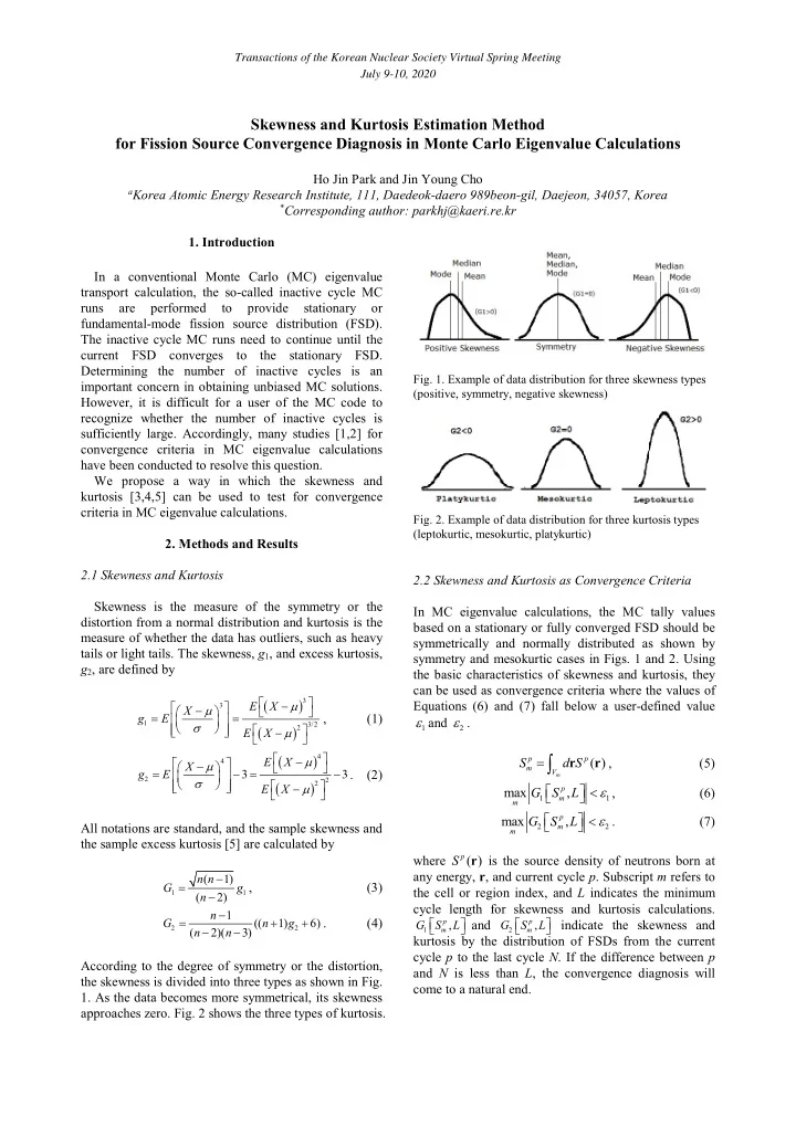
. (4) According to the degree of symmetry or the distortion, the skewness is divided into three types as shown in Fig.

• 1. As the data becomes more symmetrical, its skewness

approaches zero. Fig. 2 shows the three types of kurtosis.

• Fig. 1. Example of data distribution for three skewness types

(positive, symmetry, negative skewness)

• Fig. 2. Example of data distribution for three kurtosis types

(leptokurtic, mesokurtic, platykurtic)

2.2 Skewness and Kurtosis as Convergence Criteria In MC eigenvalue calculations, the MC tally values based on a stationary or fully converged FSD should be symmetrically and normally distributed as shown by symmetry and mesokurtic cases in Figs. 1 and 2. Using the basic characteristics of skewness and kurtosis, they can be used as convergence criteria where the values of Equations (6) and (7) fall below a user-defined value

1

 and

2

 . ( )

m

p p m V

S d S  r r , (5)

1 1

max ,

p m m

G S L       , (6)

2 2

max ,

p m m

G S L       . (7) where ( )

p

S r is the source density of neutrons born at any energy, r, and current cycle p. Subscript m refers to the cell or region index, and L indicates the minimum cycle length for skewness and kurtosis calculations.

1

,

p m

G S L     and

2

,

p m

G S L     indicate the skewness and

kurtosis by the distribution of FSDs from the current cycle p to the last cycle N. If the difference between p and N is less than L, the convergence diagnosis will come to a natural end.

Transactions of the Korean Nuclear Society Virtual Spring Meeting July 9-10, 2020

Moreover, the skewness and kurtosis estimation method can be used for judging whether MC-tally values are fully-converged or not.

1 1 m

G Q       , (8)

2 2 m

G Q       . (9) where

m

Q means any MC tally of cell m.

1 m

G Q     and

2 m

G Q     indicate the skewness and kurtosis by the

cycle-wise MC tallies from the 1st cycle to the last cycle

• N. The modules for these methods were implemented

into the McCARD MC code [6]. 2.3 Slab Test Problem To examine the effectiveness of the convergence criteria for skewness, simple slab problems were

• considered. We took the slab problem from Ref. [7] and

its cross sections are shown in Table I. The 10cm 1D slab was divided equally into ten cells. All cells had the same cross section and the leftmost (cell 1) and rightmost (cell 10) boundary surfaces of the slab had reflective boundary conditions. The dominance ratio for the slab problem was about 0.92.

Table I: Slab Problem Description

Parameter Value Total cross section(

t

 )

1.0 Scattering cross section(

,0 s



) 0.6 Production cross section (

f

v )

0.48 Width (cm) 10 Number of cell (#) 10 Initial Fission Source (FS) Uniform case /Biased case In the slab problem, all McCARD calculations were performed using 1,000 cycles (N) with 100,000 neutron histories per cycle, and no skipped cycle. The mean and standard deviation for skewness and kurtosis were calculated from 59 replicas with different random number sequences. In this study, 0.5 was used as the convergence criterion

1

 , because ±0.5 is generally considered as the acceptable range of skewness for normal distribution [8]. The other convergence criterion

2

 and the minimum cycle length L were arbitrarily set as 0.5 and 100, respectively. To examine the change of the convergence cycle length due to the initial FSD, we considered uniform and biased cases. The initial fission sources for the ‘uniform’ case were uniformly sampled from the whole slab whereas those for the ‘biased’ case were only sampled in ‘cell 1’ at the left boundary of the slab.

• Figs. 3 and 4 plot the trends of the cycle-wise

skewness and kurtosis, respectively. As the cycle proceeds, the skewness and kurtosis are closer to 0.0. Table II shows the results of convergence cycles by each method. For comparison, the convergence cycle by the Ueki’s posterior source convergence diagnosis [1] and Shim’s on-the-fly stopping criterion (Type A & B) [2] were calculated.

200 400 600 800

• 5
• 4
• 3
• 2
• 1

1 2 3 4 5

Cycle-wise Skewness CYCLE

CEL1 CEL2 CEL3 CEL4 CEL5 CEL6 CEL7 CEL8 CEL9 CEL10

0.5

• 0.5
• Fig. 3. Cycle-wise cumulative skewness of slab problem

(biased case)

100 200 300 400 500

• 4

4 8 12 16 CEL1 CEL2 CEL3 CEL4 CEL5 CEL6 CEL7 CEL8 CLE9 CEL10

Cycle-wise Kurtosis CYCLE 0.5

• 0.5
• Fig. 4. Cycle-wise cumulative kurtosis of the slab problem

(biased case)

In the ‘uniform’ case, the number of inactive cycles determined by the Ueki’s method was 3, while those by the Shim’s types A and B stopping criteria with the default option were 45 and 50. The convergence cycles

• f the uniform case by skewness and kurtosis estimation

method were 5 whereas those in the biased case were 46 and 50. Overall, we found that the convergence cycle by the new method (

1

 =

2

 =0.5) agreed well with those by the Ueki’s posterior source convergence diagnosis. Table III shows the maximum skewness or kurtosis among the results by Equations (8) and (9) for each cell. By the skewness and kurtosis estimation method, the

Transactions of the Korean Nuclear Society Virtual Spring Meeting July 9-10, 2020

MC tallies of the uniform case converged whereas those

• f the biased case did not fully converge. Fig. 5 shows

the normalized FSD of the biased case using the MC tally values from first cycle to 1,000 (=N) cycles. We

• bserved that there were considerable differences

between the MC results and the exact solutions.

Table II: Convergence cycle results for the slab problem

Method Convergence Cycle (#) Uniform case Biased case Ueki’s posterior source convergence diagnosis [1] 3 56 Type-A stopping criterion [2] 45 97 Type-B stopping criterion [2] 50 100 Skewness estimation method (

1

 =0.5, L=100) 5±1 45±3 Kurtosis estimation method (

2

 =0.5, L=100) 5±1 49±3

Table III: Skewness and Kurtosis for cumulative normalized fission source density after 1,000 cycles

Case (N=1,000) Uniform case Biased case

1 m

Max G Q    

• 0.135

(Conv.)

• 14.49

(No Conv.)

2 m

Max G Q     0.478 (Conv.) 87.57 (No Conv.)

* No Conv. = More than one MC tally values did not fully converge. ** Conv. = All MC tally values converged.

• 3. Conclusions

In this study, we introduced the skewness and kurtosis estimation methods determine the number of inactive cycles in MC eigenvalue calculations. The skewness and kurtosis estimation method determines the number of inactive cycles on the basis that fully converged FSDs may follow normal distributions without asymmetry and

• utliers. We applied the proposed methods to a simple

slab test problem. The results confirmed that the skewness and kurtosis estimation method reasonably determined the convergence cycle under the current convergence criteria (

1

 =

2

 =0.5). The proposed method will be very useful for determining the number

• f inactive cycles and judging whether MC tally values

are fully converged. Meanwhile, the OECD/NEA working group released the slow source convergence benchmark program [8] to solve the slow convergence problem combined with statistical fluctuations. In the near future, the skewness and kurtosis estimation methods will be applied to the slow convergence benchmark problem to examine their performance and reliability.

1 2 3 4 5 6 7 8 9 10 0.94 0.96 0.98 1.00 1.02 1.04 1.06

Normalized Fission Source Density Cell index Exact Solution (=1.0)

• Fig. 5. Cumulative normalized fission source density after

1,000 cycles in slab problem (biased case)

REFERENCES

[1] T. Ueki, F. B. Brown, “Stationarity modelling and informatics-based diagnostics in Monte Carlo criticality calculation,” Nucl. Sci. Eng., Vol.149, p. 38, 2005. [2] H. J. Shim, C. H. Kim, “Stopping criteria of inactive cycle Monte Carlo calculations,” Nucl. Sci. Eng., Vol.157, p. 132, 2007. [3] T. A. Jones, “Skewness and Kurtosis as criteria of normality in observed frequency distributions,” Journal of Sedimentary Research, Vol.39, p.1622, 1969. [4] T. J. Trahan, “Region-Specific Monte Carlo Analysis of Stochastic Systems,” Trans. Am. Nucl. Soc., Vol.119, Nov. 11-16, 2018, Orlando, FL, USA. [5] D. N. Joanes, C. A. Gill, “Comparing Measures of Sample Skewness and Kurtosis,” The Statistician, Vol.47, 1, p.183, 1998. [6] H. J. Shim et al., “McCARD: Montel Carlo code for advanced reactor design and analysis,” Nucl. Eng. Tech., Vol. 44, p.161, 2012. [7] H. J. Park, H. C. Lee, “Application of Higher Order Fission Matrix for Real Variance Analysis in McCARD Monte Carlo Eigenvalue Calculation,” M&C2017, Apr. 16-20, 2017, Jeju, Korea. [8] M. G. Bulmer, Principles of Statistics, Dover, 1979. [9] R. N. Blomquist, A. Nouri, “The OECD/NEA Source Convergence Benchmark Program,” Trans. Am. Nucl. Soc., Vol.87, 142, 2002. Transactions of the Korean Nuclear Society Virtual Spring Meeting July 9-10, 2020