Deep Learning for Computational Science and Engineering Jeff Adie - - PDF document

Deep Learning for Computational Science and Engineering Abstract

Recent advancements in the field of Artificial Intelligence, particularly in the area of Deep Learning have left many traditional users of HPC somewhat unsure what benefits this might bring to their particular domain. What, for example, does the ability to identify members of felis catus from a selection of uploaded images on Facebook have to do with modeling the oceans of the world, or discovering how two molecules interact? This paper is designed to bridge the gap by identifying the state-of-the-art methodologies and use cases for applying AI to a range of computational science domains. Keywords AI, Deep Learning, Computational Science, HPC 1. Introduction Artificial Intelligence (AI) is considered to be a key enabler

• f the fourth Industrial Revolution [1] and, as such, a game-

changing technology. AI is a very broad field, and in the context of this paper, we restrict ourselves to a subset of Machine Learning (ML), which in of itself is a subset of AI. That subset is based on the application of Artificial Neural Networks (ANN) and, in particular Deep Neural Networks (DNN). Whilst AI has been around for many years, three key events have come together to cause this “perfect storm” and allow the application of DNNs (referred to as Deep Learning) to become practical. The first of these events was the development of newer algorithms in the 2000s. Secondly,

• ur interconnected world provided the huge amounts of data

required to train neural networks effectively. Thirdly, the hardware technology, and in particular the use of GPUs for processing neural networks, made multi-layer networks with multiple hidden layers possible. All these three things came together in 2012, when Alexnet [2] became the first DNN to win the imageNet 2012 comptetition (an image classification challenge). Since that time, the field has exploded with deeper networks, faster GPUs and more data available. For example, the original AlexNet was 8 layers deep, but state of the art networks can be hundreds or even thousands of layers deep [3]. Our purpose in undertaking this survey is not so much to understand how these DNNs work, but rather how they can be applied to solve various, important real world tasks in the field of Computational Science. One area we decided not to survey was the role in life sciences of medical imaging as we felt there was an implicit understanding that operations such as image classification, segmentation and object detection were both obvious and well understood. 2. Classification Taxonomy methodology There are many different approaches that we considered in determining how to classify the application of AI to Computational science. One approach is to consider specific applications in which AI has been incorporated. Another is to classify the research by domains. There is also the consideration of numerical methods which apply across domain and application spaces, in a similar vein to Colella’s Dwarfs [4], or the Berkely Dwarfs [5] The approach we decided on was to classify by domain space, setting out five major domains and then subdividing each of these into more specific application segments, and then calling out specific applications where appropriate. Jeff Adie Nvidia AI Technology Center, Singapore jadie@nvidia.com Yang Juntao Nvidia AI Technology Center, Singapore yjuntao@nvidia.com Xuemeng Zhang Nvidia AI Technology Center, Australia maggiez@nvidia.com Simon See Nvidia AI Technology Center, Singapore ssee@nvidia.com

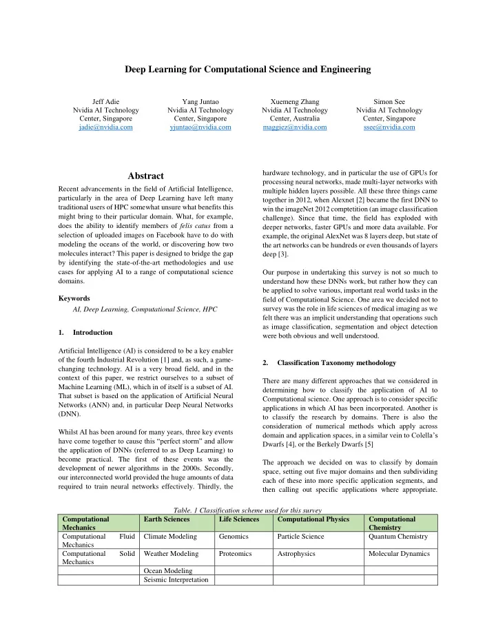
• Table. 1 Classification scheme used for this survey

Computational Mechanics Earth Sciences Life Sciences Computational Physics Computational Chemistry Computational Fluid Mechanics Climate Modeling Genomics Particle Science Quantum Chemistry Computational Solid Mechanics Weather Modeling Proteomics Astrophysics Molecular Dynamics Ocean Modeling Seismic Interpretation

Table 1 below lists the major domains and sub-domains. To ensure coverage of cross-domain numerical methods as well, we have included an additional section dedicated to that. 3. Computational Mechanics 3.1. Computational Fluid Mechanics Deep learning was a huge breakthrough in data mining and pattern recognition. Its recent success has been mostly limited in imaging and natural language processing. However, it is expected that deep learning’s success will soon be extended to more applications. J. Nathan Kutz has predicted, in his article published in Journal of Fluid Mechanics, that deep learning will soon make their mark in turbulence modelling, or general area of high-dimensional, complex dynamical systems. [6] Compared with traditional machine learning method, J Nathan Kutz believes that DNN are better suited for extracting multi-scale features and handling of translations, rotations and other variances. [6] Even though the performance gain is based on large increase

• n computational cost for training, development of modern

hardware like GPU could potentially accelerate the training to take full advantage of the DNN. There has already been some published work on attempts of deep learning for computational fluid dynamics. Direct application of deep learning for quick estimation of steady flow has been investigated by researchers and companies like Autodesk. [7] Such direct application of deep learning as a mapping function can be found in many other computational domains as well, it generally provides huge acceleration for computational complex problems with certain trade off in accuracy. Besides accelerating traditional numerical methods, deep learning has also find its application in computational fluid dynamics frontier. A research group from University of Michigan has been investigating on data driven method for turbulence modelling. As a result, an inverse modelling framework was proposed, and a few machine learning techniques has been tested and compared under the

• framework. [8] [9] [10] [11]. On top of their work, Julia Ling

from University of Texas proposed a specific DNN instead

• f traditional machine learning with promising results. [12].

Besides the academia, Industrial leaders like GE are also investigating the potential of data-driven methods. GE has recently publishing their latest achievement on machine learning techniques for turbulence modelling with collaboration from University of Melbourne. [13] In addition to CFD researchers’ attempts, there are researchers from computer graphics domain also demonstrated progressive research work on deep learning for fluid simulation. And it has already shown its capability in accelerating fluid simulations in real time interactive

• schemes. Computer Graphics Lab of ETH is one of the few

early explorers. They considered the traditional problem as a regression problem and accelerated them with machine

• learning. [14] Classical SPH method was used to generate

training data for regression forests training. The trained regression forest would be able to inference the acceleration

• f particles in a real time fluid simulation much faster. Some
• ther researchers approached from the Eulerian fluid

simulation instead. Successful research works has shown that trained Convolutional Neural Network (CNN) is able to accelerate the pressure projection step in the Eulerian fluid

• simulation. [15] Similar work has also been published on

ICML 2017. The experimental results have confirmed such methods are capable of not only accelerating the simulation but also achieve comparative accuracy. [16] In addition to the works mentioned above, there are other researchers believe solving sub-problems of Naiver-Stokes’ equation by coupling deep learning is a better approach than trying to solve NS equation directly by trained neural

• networks. Deep learning is used in Mengyu Chu’s work on

smoke synthesis. [17] CNN is trained to pick up information from advection-based simulation and match them with data from pre-exist fluid repository to generate more details of smoke with faster speed. Kiwon Um utilized similar tactics in liquid splash modelling. [18] In his work, a neural network is used to identify regions where splash took place from FLIP simulation data. Then droplets are generated in those regions to improve the visual fidelity. There will certainly be more researchers and engineers make use of deep learning in fluid dynamics research. Such practice and trends will bring more awareness of statistics and data science culture into fluid dynamics community. A proper data set for training and testing of upcoming more DNN based architectures would be helpful in standardizing fair comparison. [6] 3.2. Computational Solid Mechanics Similar to the application of deep learning techniques in fluid simulations, researchers from the computational mechanics domain are also exploring the potential of machine learning. There was many researches work done by updating FEA model with traditional machine learnings. The application has been found in modeling the constitutive modeling of material, FEA model updating and mesh generation/refinement and etc. [19] [20] [21] [22] [23] Deep learning based method has also been applied in FEA model

• update. Some has been tested in medical applications. One

published paper from Spain has demonstrated how to train random forests with FEA based solver to model the mechanical behavior of breast tissues under compression in real-time. [24] Jose D. Martin-Guerrero applied similar techniques for modeling of biomechanical behavior of

human soft tissue. [25] Similar technique is also used in Liang L’s deep learning approach of stress distribution

• estimation. [26] There is also a spin off called deepvirtuality

started from BMW Data:Lab. Based on FEA data trained neural network, it is able to predict structural data in real

• time. It provides much quicker alternative than FEA solvers

in early design stage. Due to the maturity of Finite Element Method itself in the solid mechanics domain, the direct application of deep learning to replace FEM methods is limited, it mostly focuses on speeding up and give a faster design evaluation in the early stage. However, there are some other ways of making use of deep learning in solid mechanics simulation, especially to make use of its strength in classification. Spruegel used deep learning to accelerate the checking of plausibility of FEA simulation which otherwise must be done with very experienced engineers. [27] Deep learning has also been extensively used in structural defect detections and etc with its successful techniques in computer vision. 4. Earth Sciences The domain of Earth sciences encompasses studies of our planet and its composition, from the earth itself (seismology, geography) through to the atmosphere (climate, weather). A large component of earth sciences is modeling and simulation for predictive purposes. Furthermore, as the capability of the hardware has progressed, more and more frequently we see a combination of modeled systems coupled together to provide an integrated solution. These coupled systems are generally referred to as earth systems. For our purposes, we break the domain into two segments somewhat whimsically referred to ‘above ground’, and ‘below ground’. Here, above ground refers to processes

• ccurring in the atmosphere or oceans of the world, and

below ground refers to subterranean events. 4.1. Climate, Weather and Ocean Modeling (CWO) 4.1.1. Climate Modeling Climate modeling refers to the study of the earth’s weather

• ver a long period of time, typically multi-year or multi-

decadal periods, in order to predict future trends for various variables, such as temperature, CO2 concentration, Ocean salinity, etc. By it’s very nature, climate studies consist of vast amounts of data with observational data going back over many decades to be considered. This makes it an ideal candidate for Deep learning There are numerous cases where DNN can be applied to climatic data. Techniques such as anomaly detection through autoencoders and classification DNNS can be applied to massive climate datasets to find such occurrences as extreme weather events [28]. This solves a task that is extremely difficult and error-prone previously. Another example is using deep learning for downscaling climate variables as described by Moutai et al [29]. This is particularly relevant in climate because often the earlier records have less data, or even no data at certain locations. As climate data is time-series based, DNNs are also a natural fit for spatiotemporal analysis, with the work of Seo et al [30] in using a graph convolutional autoencoder in conjunction with a Recurrent neural networks (RNN) as a good example. As they point out, meteorological measurements are significantly dependent on location, and so it is important to engage in both space and time. In their case, using the autoencoder for extracting spatial features, and the RNN for temporal positioning. 4.1.2. Weather Modeling Weather modeling, usually referred to as numeric weather prediction (NWP), is similar to climate modeling, but concerns short-term forecasting of future weather from immediate (nowcasting) up to 10 days or so. NWP is not

• nly used for the development of weather forecasts, but also

as atmospherics drivers for modeling forest fires, air pollution, energy budgets (solar, wind) and so forth. NWP is

• ne of the largest users of HPC cycles outside of the national

labs. One key application for Deep Learning in NWP is the prediction of tropical cyclones. Here, the work by Matsuoka et al [31] is a very good example. They trained an ensemble

• f CNNs with over 10 million images and 2,500 typhoon

tracks, achieving a > 87% accuracy and a 2-day prediction window ahead of satellite observation data. Another important application is the prediction of

• precipitation. Kim et al [32] showed in their Deep Rain

design how a stacked network of convolution / long short- term memory (LSTM) nodes could accurately predict rainfall after being trained on 2 years of weather radar data with a RSME of 11%, which was 23% better than any previous effort. An interesting approach taken by one commercial company, Yandex, combines traditional NWP with deep learning and local observations to provide a personalized hyper accurate

• forecast. This system is constantly self-adjusting, comparing

itself against actual values and incrementally improving, making 140000 comparisons each day with over 9 TB of input data [33]. 4.1.3. Ocean Modeling Ocean modeling covers the study of the ocean and the coastline from both an ecological as well as a physical

• aspect. Ocean modeling is often used to model the sea

currents, ocean salinity, chemical concentrations, erosion,

• etc. The modeling of sea ice for polar regions is also

considered a part of ocean modeling. Many systems employ a separate wave model, which is then coupled to a deep

• cean model (and possible an atmospheric model as well).

A good early piece on generating Ocean salinity and temperature values was given by Bhaskaran, et al [34], which showed that a MLP with an appropriate backpropagation algorithm was able to derive salinity and temperature values at any desired points with a high degree

• f accuracy. In a similar vein, Ammar et al’s work [35]

determined sea surface salinity from satellite brightness temperatures using a deep learning system with high accuracy by deploying multiple networks to derive an ensemble result with 97% of the tests showing a bias less than 0.2 psu. Deep learning has been employed to provide rapid forecasts

• f wave conditions as discussed in [36] and [37] , and is now

capable of providing extremely good results with the recent work of James, et al [38] giving a small (RSME < 9cm) error with 1000x speedup over the traditional method of modeling the energy in the waves directly. In their example, they use two different models with a MLP to perform regression analysis on the wave height, and a second component to classify the characteristic period of the wave. Deep learning is also valuable for the use of super-resolution

• f satellite data in ocean modeling. A good example of this

is given in [39], whereby sea surface temperature (SST) data is taken from satellite data up downscaled to the model grid. The use of a SRCNN network improved the quality of the

• utput substantially compared to traditional interpolation

filter techniques. 4.2. Seismic Modeling and Interpretation Whilst this field has several areas of interest, we are focusing

• n seismic interpretation and modeling as a key field due to

the importance of this field in the HPC community. Seismic processing is the largest commercial use of HPC in the world and is a key part of the exploration chain in the oil & Gas

• industry. It has been suggested by McKinsey [40] that more

than $50 Billion in savings and operational improvements could be realized in upstream processing alone from AI. It is also an important field for the monitoring and detection of naturally occurring seismic events, such as earthquakes and eruptions. One interesting work by Bhaskar & Mao [41] utilized Deep Learning for the purpose of Automatic Fault interpretation. They showed after training with 2.5 million expertly labelled images, they were able to detect key fault features in seismic records with an accuracy of 81%. In another example, Waldeland & Solberg [42] used a CNN to interpret 2D slices for salt deposits and extended that to extracting 3D models of the salt deposits, showing the generality of the discriminator from one slide to all slices. One very recent study from Harvard [43] showed a 20x improvement in earthquake detection through the use of a CNN called ConvNetQuake. This network can detect seismic events orders of magnitude faster than traditional methods. 5. Life Sciences Research in life science has been driven from algorithm- centric to data-centric by high-throughput technologies. The data explosion is challenging for traditional methods to extract and interpret useful information from the vast amount

• f structured, semi-structured, weakly structured, and

unstructured data. Deep learning has been revolutionizing the research in life science. Scientists have adapted deep learning to the tasks of a variety of life science applications and it has demonstrated high accuracy and strong portability over existing methods. Various deep learning algorithms have their own advantages to resolve particular types of problems in life science

• applications. For example, CNNs have been widely adopted

to automatically learn local and global characterization of genomic data. RNNs are skillful at handling sequential data such as protein sequences. Autoencoders are popular for both pre-trained models and denoising or preprocessing the input data [44]. In this section, we provide a concise review of the state-of-the-art methods that are based on deep learning in genomics and proteomics, respectively. 5.1 Genomics Genomic research aims to understand the genomes of different species. It studies the roles assumed by multiple genetic factors and the way they interact with the surrounding environment under different conditions [44]. Genomics is becoming increasingly data-intensive due to the high- throughput sequencing (HTS) technology. DNNs offer a new promising approach for analysis of genomic data, through their multi-layer representation learning models. 5.1.1. Predicting enhancers and regulatory regions Identifying the sequence specificities of DNA- and RNA- binding proteins is the key to model the regulatory processes and discover causal disease variants. Using modern high- throughput technologies, this problem is computationally demanding as the quantity of data is large, and traditional techniques have their own uncertainties, biases, artifacts, and generate different forms of data. To address this problem, a deep learning approach, DeepBind [45], has been developed

and applied to both microarray and sequencing data and learn from millions of sequences of the tested proteins accurately and efficiently. DeepBind uses deep CNNs and can train the predictive models fully automatically. The training stage can be accelerated on NVIDIA GPUs for 10-70x speedup and the trained models can be deployed on CPUs, which is flexible and scalable. Specificities determined by DeepBind can be visualized as a weighted ensemble of position weight matrices (PWM) or as a “mutation map” that indicates how variations affect binding within a specific sequence. For training, DeepBind learns several levels of representation

• f the input sequence to predict the protein-binding score. It

uses a set of sequences of varying lengths, and for a sequence, it computes a binding score using four stages: convolution, rectification, pooling, fully connected layers. The sequence is encoded by a binary matrix of size n * 4 where n is the sequence length and 4 rows represent A,C,G,T respectively. The convolutional layers transform the matrix into feature vectors which capture local sequence patterns of different

• motifs. The rectification stage isolates positions with a good

pattern match by shifting the response of motif detector and clamping all negative values to zero. The pooling layers compute the maximum and average of the feature vectors, then the values are fed into fully connected layers to compute the output of the model. The output score is compared to the target and the error signal is used to tune the weights of neural network using backpropagation. One important problem within genetic sequence understanding is related to transcription factors (TFs) which are regulatory proteins that bind to DNA. Each TF binds to specific transcription factor binding sites on the DNA sequence to regulate cell machinery. Deep Motif [46] focuses

• n accurately classifying whether there is a binding site for a

specific TF given an input DNA sequence, using a deep convolutional and highway multi-layer perceptron (MLP)

• network. It also can extract motifs, or symbolic patterns

which are visual representations of positive binding sites for a particular TF. Experiments show that Deep Motif extracts motifs that similar to, and in some cases outperform the previous well know motifs. Compared to DeepBind [45], Deep Motif has a deeper network, thus achieving a higher area under the curve (AUC) for 92 out of 108 TF datasets and a higher median AUC score. Identifying functional effects of noncoding variants is a major challenge in human genetics. To predict the noncoding- variant effects de novo from sequence, a deep learning-based algorithmic framework DeepSEA [47] has been developed, which directly learns a regulatory sequence code from large- scale chromatin-profiling data, including TFs binding, DNase I sensitivity and histone-mark profiles. DeepSEA can predict the chromatin effects of sequence alterations with single- nucleotide sensitivity. It can accurately predict the epigenetic state of a sequence, including TFs binding, DNase I sensitivities and histone marks in multiple cell types, and further utilize this capability to predict the chromatin effects

• f sequence variants and prioritize regulatory variants.

Zeng et al. [48] present a systematic exploration of CNN architectures for predicting DNA sequence binding using a large compendium of TF datasets. They identify the best- performing architectures by varying network width, depth and pooling designs, and vary each of these dimensions while

• bserving

classification performance

• n

each TF

• independently. For the two tasks, motif discovery and motif
• ccupancy, classification performance increases by adding

convolutional kernels. CNNs that take advantage of these insights exceeded the classification performance of DeepBind [45], which represents one particular point in the parameter space. The benefits of CNNs are learning rich higher-order sequence features, such as secondary motifs and local sequence context, by comparing network performance

• n multiple modeling tasks ranging in difficulty. In addition,

careful construction of sequence benchmark datasets, using approaches that control potentially confounding effects like positional or motif strength bias, is critical in making fair comparisons between competing methods. They explore how to establish the sufficiency of training data for these learning tasks, and they have created a flexible cloud-based framework that permits the rapid exploration of alternative neural network architectures for problems in computational biology. In double-stranded DNA, the same pattern may appear identically on one strand and its reverse complement due to complementary base pairing. Conventional deep learning models that do not explicitly model this property can produce substantially different predictions on forward and reverse- complement versions of the same DNA sequence. Shrikumar et al. [49] present four new CNN layers that leverage the reverse-complement property of genomic DNA sequence by sharing parameters between forward and reverse- complement representations in the model. These layers guarantee that forward and reverse-complement sequences produce identical predictions within numerical precision. Using experiments on simulated and in vivo TF binding data, their CNN architectures lead to improved performance, faster learning and cleaner internal representations compared to conventional architectures trained on the same data. In genomics, the same positional patterns are often present across multiple convolutional channels. Therefore, there exists significant redundancy in the representations learned by standard fully connected layers. Alexandari et al. [49] present a new separable fully connected layer that learns a weights tensor that is the outer product of positional weights and cross-channel weights, thereby allowing the same positional patterns to be applied across multiple convolutional channels. Decomposing positional and cross- channel weights further allows imposing biologically- inspired constraints on positional weights, such as symmetry. They also propose a novel regularizer and constraint that act

• n curvature in the positional weights. Using experiments on

simulated and in vivo datasets, the networks that incorporate their separable fully connected layer

• utperform

conventional models with analogous architectures and the same number of parameters. Additionally, their networks are more robust to hyperparameter tuning, have more informative gradients, and produce importance scores that are more consistent with known biology than conventional DNNs. 5.1.2. Gene Expression Gene expression analysis provides quantitative information about the protein and mRNA abundance across the whole

• rganism and in the individual tissues and cells. Capturing

the gene expression patterns can help studying molecular mechanisms implicated in diseases and cellular responses to drug treatment. One of the first computational steps in exploration and analysis of the gene expression data is

• clustering. With a number of standard clustering methods

routinely used, most of the methods do not take prior biological information into account. Cui et al. [51] propose a new approach for gene expression clustering analysis, which combines an autoencoder method with the prior biological

• knowledge. The first stage uses Robust Autoencoder, which

provides a more accurate high-level representation of the feature sets. Once the network is trained, the low dimensional representation of the gene expression profile is used for the clustering task. The second stage defines a network-based metric which allows introducing the community information

• f each gene in the network into the clustering process, based
• n the hypothesis that two genes in the same network

community are more likely to share the same expression

• pattern. This approach has been tested on two distinct gene

expression datasets and it outperforms two widely used clustering methods, hierarchical clustering and k-means, as well as a recent deep learning autoencoder approach. 5.1.3. Variant calling HTS can generate a huge amount of short sequences, and processing the HTS output into a single, accurate and complete genome sequence is a outstanding challenge. Hand- crafted and parameterized statistical models used for variant calling still produce thousands of errors and missed variants in each genome. DeepVariant [52] is a universal SNP and small indel variant caller created using DNNs. It transforms the task of variant calling into an image classification problem and applies to Tensorflow framework. DeepVariant can reconstruct the true genome sequence from HTS sequencer data with significantly more accurate than previous

• methods. The learned network can also generalize across

genome builds and even to other species than human. The deep learning model has no specialized knowledge about genomics or next-generation sequencing. The reads relevant for a putative variant are piled up and presented as an RGB image, then fed into a CNN which learns statistical relationships between images of reads and ground-truth genotype calls. Initial CNN can be a random model, a CNN trained for other image classification tests, or a prior DeepVariant model. Labeled images and genotype pairs are used to optimize the CNN parameters to maximize genotype prediction accuracy using a stochastic gradient descent

• algorithm. After certain training time or convergence, the

final trained model can be used for variant calling. 5.1.4. Methylation DNA methylation is one of the most extensively studied epigenetic marks and is known to be implicated in a wide range of biological processes. Most existing methods for predicting average DNA methylation do not take cell-to-cell variability into account. They also require a priori defined features and genome annotations which are typically limited to a narrow set of cell types and conditions. DeepCfG [53] is a computational approach based on DNNs to predict single cell methylation states and model the sources of DNA methylation variability. Unlike previous methods, it leverages associations between DNA sequence patterns and methylation states, as well as between neighboring CfG sites, both within individual cells and across cells. Experimental results show that DeepCpG has yielded substantially more accurate predictions of methylation states than previous

• approaches. In addition, it has unveiled de novo sequence

motifs that are associated with methylation changes and methylation variability between cells. DeepCpG has a CpG module to consider correlations between CpG sites within and across cells, a DNA module to detect informative sequence patterns, and a Joint module to combine the output of CpG and DNX module to predict methylation states at target CpG sites. The CpG module is based on a bidirectional gated recurrent network, scans the CpG neighborhood of multiple cells, yielding compressed features in a vector of constant size. The DNA module uses two convolutional and pooling layers to identify predictive motifs from the local sequence context and one fully connected layer to model motif interactions. Finally, the Joint module learns interactions between higher-level features derived from the two modules to predict methylation states in all cells. The trained model can be used for different downstream analyses, including genome-wide imputation of missing CpG sites, and discovery of DNA sequence motifs that are associated with DNA methylation levels or cell-to- cell variability. 5.1.5. Single-cell applications Mass cytometry or CyTOF is an emerging technology for high-dimensional multiparameter single cell analysis. Gating (assigning individual cells into discrete groups of cell types) is one of the important steps and bottleneck of analyzing CyTOF data. It involves time-consuming sequential manual steps untenable for larger studies. The subjectivity of manual gating introduces variability into the data and impacts reproducibility and comparability of results, particularly in multi-center studies. DeepCyTOF [50] is a deep learning

approach for gating based on a multi-autoencoder neural

• network. It employs one manually gated reference sample

and utilizes it for automated gating of the remaining samples. DeepCyTOF is based on domain adaptation principles and is a generalization of previous work that allows to calibrate between a source domain distribution (reference sample) and multiple target domain distributions (target samples) in a supervised manner. It has been applied to two CyTOF datasets generated from primary immune blood cells, and achieves high concordance (99%) of the cell classification

• btained by individual manual gating. Additionally, a stacked

autoencoder, which is one of the building blocks of DeepCyTOF, combined with a domain adaptation procedure,

• ffer a powerful computational approach for semi-automated

gating of CyTOF and flow cytometry data such that manual gating of one reference sample is sufficient for accurately gating the remaining samples. 5.2. Proteomics Proteomics focuses on large scale studies to characterize the proteome, the entire set of proteins, in a living organism [51]. This section demonstrates the advantages of new data-centric approaches powered by deep learning technology over traditional methods in two proteomic areas: de novo peptide sequencing and protein structure prediction. 5.2.1. De novo peptide sequencing In proteomics, de novo peptide sequencing from tandem mass spectrometry data plays the key role in characterization of new protein sequences. The task of de novo peptide sequencing is to reconstruct the amino acid sequence of a peptide [51]. DeepNovo [52] is the first deep learning model for de novo peptide sequencing. DeepNovo architecture combines two CNNs and a LSTM network to learn features

• f tandem mass spectra, fragment ions, and sequence patterns
• f peptides. The first CNN learns local alternative peak

features of all possible next amino acid candidates, while the second CNN learns general features of the spectrum and pass them to the LSTM network. The LSTM network learns sequence patterns of the currently predicted partial peptide in association with the spectrum features from the second CNN. The information from the first CNN and LSTM networks are combined to make the final decision. DeepNovo has been developed on Tensorflow and accelerated by NVIDIA Tesla P40 GPU. Evaluation results show that DeepNovo has outperformed other approaches on a wide variety of species, achieving higher accuracy at amino acid level and peptide level. DeepNovo can also automatically reconstruct the complete sequences without assisting databases. Furthermore, DeepNovo is retrainable to adapt to any sources of data and provides a complete end-to- end training and prediction solution to the de novo sequencing problem. 5.2.2. Protein structure prediction Information of protein contacts are crucial for the understanding of protein structure and function. Direct evolutionary coupling analysis (DCA) for protein contact prediction is only effective on proteins with a large number (>1000) of sequence homologs, therefore, predicted protein contacts of small number (<134) of sequence homologs is of low quality and not useful for de novo structure prediction [53]. To improve contact prediction, Wang et al. [53] [54] [55] have developed a novel deep learning method which can improve contact prediction accuracy greatly, regardless of the sequence homolog number for a protein. Although there are many challenges, they have transferred the knowledge in computer vision to contact prediction, by treating a protein contact map as an image and protein contact prediction as pixel-level image labeling. This method employs a deep residual neural network consisting of two neural networks. It can automatically learn the complex relationship between sequence information and contacts, also model the dependency among contacts which improve contact prediction. The first network includes a series 1D convolutional transformation of sequential features, the output of the first network is converted to a 2D matrix by

• uter concatenation, then fed into the second network with

pairwise features. The second network conducts a series of 2D convolutional transformation, followed by a logistic regression to predict the probability of any two residues form a contact. Experimental results show that contacts predicted by this method can achieve higher accuracy and more accurate contact-assisted folding. In addition, this method has been applied to predict protein contact in CASP12 [54]. It is also the first method that can predict membrane protein by learning from non-membrane proteins [55]. Furthermore, this deep learning method will also be useful for the prediction of protein-protein and protein-RNA interfacial contacts [53]. 6. Computational Chemistry Computational Chemistry is the use of computer models and computer simulation to study the chemical properties of

• molecules. These models tend to be exponentially difficult

to solve with size and generally cannot be solved

• analytically. In general, the field can be divided by the

method used to simulate the chemical process, with techniques based on quantum mechanics (so called ab initio methods) where the electronic structure of the molecule is critical, as opposed to semi-emperical methods whereby the dynamics of the molecules over time is more important. However, we note that with modern processing power and application of AI, there is more crossover between QC and

• MD. As an example, consider ab-initio Molecular Dynamics

AIMD, where QC methods are used for MD.

We would be remiss if we did not mention the work of Goh, et al [56] in solidly covering the ground of Deep Learning research in this domain. This paper is a comprehensive survey of computational chemistry and well worth reading for anyone working in this field. To avoid repetition and therefore redundancy, we have tried to concentrate on research since this publication or not covered in their paper. 6.1. Quantum Chemistry To begin our foray into QC, we note the work of DeepChem [57] and MoleculeNet [58]. The open source DeepChem package is deep learning framework for drug discovery based on python and tensorflow. MoleculeNet is provides a mechanism to train/validate/test and benchmark 17 datasets containing over 700,000 curated compounds using DeepChem, 4 of which are based on quantum mechanics. It provides mechanisms to smartly spilt datasets (as traditional naïve approached such as random splits are often not suitable for chemical data), as well as a number of featurization methods (for encoding molecules into fixed length vectors) and models to compare. Garrett Goh and his team from PNNL who provided the comprehensive survey of the field of Computational Chemistry noted in [56] have also come up with Chemception [59]. This is a CNN, inspired by the Inception- ResNet [60] from Google for Image classification, that can classify molecules from 2D drawings. They showed a single NVIDIA GTX 1080 could train the complex HIV model within 24 hours, providing comparable performance for toxicity, activity and solvation predictions to current QSAR/QPSR models. Another recent advance is in the use of multiscale invariant dictionaries by Hirn, et al [61] in order to estimate quantum chemical energies which requires a fraction of the computational expense of calculating the bond energies, and yet are as accurate as standard DFT functions. 6.2. Molecular Dynamics Schutt, et al [62] have showed that, with their deep tensor neural network (DTNN), they have the ability to predict the chemical space for molecules of intermediate sizes with a uniform accuracy of 1 kcal/mol, which is considered the commonly acceptable limit for chemical accuracy. They do this in a similar fashion to CNNs, by taking advantage of the ability to capture local structure. In a similar vein, but with ab initio MD (AIMD) in order to include vibrational anharmonic and dynamical effects that are normally ignored, the work of Gastegger, et al [63] shows both a high order of accuracy in the NN result Zhang, et al [64] showed how DNN could provide AIMD quality with markedly improved performance through a Deep Potential Molecular Dynamics (DeePMD) DNN that

• vercomes

the usual problems

• f

translational/rotational/permutational symmetry by assigning a local reference frame to each atom. Their paper shows results scaling linearly up to 105 molecules and three

• rders of magnitude faster than AIMD performed using

Quantum Espresso. Related to DeePMD and largely from the same authors, the work of Wang, et al [65] in developing DeePMD-kit should be noted, as it provides an interface between Deep learning representations of energy (based on Tensorflow) and traditional MD Simulations (based on LAMMPS). This work allows the training to be simply and efficiently applied to MD simulations. 7. Computational Physics Computational physics is one of the three corner stones for physics research together with theorem and experiments. Traditional computational physics has been most relied on numerical methods to solve physical equations. However, due to the data-intensive nature of many physics study, deep learning has slowly become an alternative option for computational physicists. Like the research in CFD domain, physicists also explored CNN-based CFD surrogate model for direct generation of solutions to steady state heat conduction and incompressible fluid flow. [66] A conditional Generative Adversary Networks was used to learn directly from experimental observations for the surrogate model to deal with problems that underlying physical model is complex and unknown. The computational performance is also improved since inference stage does not take much computation. Physicist at the Large Hadron Collider (LHC) are also investigating adoption of deep learning where traditionally they rely on computational simulation of particle collisions. [67] GAN-based methods named CALOGAN is used to model the physical sequential dependence among the calorimeter layers which provides a speed-up to a factor of 100,000 times. Deep learning also found its place in solving the Schrodinger equation. A specific CNN has been used to map 2D Schrodinger equation problem from 2D potentials to an electron’s ground-state energy. [68] Besides those attempts to use deep learning for physics based computational simulation, there are also frequent usage of deep learning in the signal/event detection from the complexed experimental results. Success stories can be found in a wide range from LHC particle research to the detection of gravitational wave. [69] [70] [71] 8. Cross-domain numerical methods 8.1. Partial Differential Equations (PDEs) PDEs are a fundamental numerical method used in many disciplines from Weather forecasting to Fluid Dynamics to

• Astrophysics. A considerable body of work has gone into

looking at using ANNs to solve various PDEs more quickly and accurately than by using traditional numerical methods. A seminal breakthrough was the work by Lagaris, et al [72] which provided a method to separate the boundary conditions from the ANN, effectively unconstraining the neural network component from initial/boundary values. A standard technique for solving a specific PDE is to formulate a weak function and use that as the loss function for a standard MLP network. See [73], [74], [75], [76], [77] as typical examples. This works well for specific PDEs but requires the development of the trial function on a case by case basis. This makes it unsuitable for general solutions. Another approach is to try to learn the PDE from data, as exemplified in [78] using a deep feed forward network, loosely modeled on the standard ResNET, but using temporal blocks to solve time dependent step non-linear

• dynamics. In a similar vein, but with a substantially different

method, the PDE-FIND [79] works by creating a large library of candidate terms for the data and derivatives and selects a sparse subset of active terms from this list. Yet another approach is to use reinforcement learning as proposed in [80] whereby the PDE is formulated as a backward stochastic differential equation (BSDE) and the gradient of that BSDE plays the role of the policy function for a RL DNN. A similar approach is also noted in [81] specifically for 2nd order nonlinear PDEs and 2nd Order BSDEs, which introduced the deep 2BSDE method that utilizes a temporal forward discretization plus a spatial approximation via DNNs. Finally, of interest is the technique of Constrained Back- propagation (CPROP) as detailed by Ferrari & Jensenius in [82], and applied to PDEs in [83] and [84]. In particular, the last paper details a Constrained Integration approach that allows for irregular grid initial value problems, which is a typically difficult class of problems to solve. 8.2. N-Body Problems N-body problems describe the interrelationship between various objects (particles or bodies) and are notoriously expensive to model as N increases. Whilst improved techniques for handling N-body interaction have been developed, such as the Barnes-Hutt or Fast Multipole methods that can improve solution times from O(N2) to O(N log N), it is still a computationally expensive operation. Indeed, todays best supercomputers can solve the wave equation exactly for n-body systems with a maximum value

• f n=45 and that a system of n=273 would require a

computer with more bits than there are atoms in the universe [85]. N-body problems occur in many fields from astronomy to quantum chemistry. An early seminal paper on solving N-Body problems thorough the use of deep learning is by Quito, et al [86]. More recently, Lam and Kipping [87] showed that a DNN trained on N-Body simulations could significantly improve stability predictions for complex planetary configurations. Another approach taken is to use reinforcement learning as shown by Carleo & Troyer [88] to solve the wave function. Gao and Duan [89] meanwhile tackle the number of parameters required, arguing that a DNN can efficiently represent that states while a shallow Restricted Boltzmann Machine (RBM) style of neural network cannot. It should also be noted that Hirn, et al’s work [61] as previously cited is also relevant here. 8.3. Monte Carlo Techniques Monte Carlo methods cover a range of algorithms that incorporate randomness to obtain results. These methods are used for optimization problems, numerical integration problems and many other types of problem where other more deterministic approaches would be too difficult. One variation on Monte Carlo methods is the Self-Learning Monte Carlo (SLMC) whereby the simulation is sped up through the use of an ‘effective model’ of the system, which is significantly faster to simulate. The problem is that the effective model needs to be human-designed. Shen et al [90] proposed a system whereby a DNN can used for the effective model, providing a similar level of accuracy, and speedup from O(N2) to O(N log N). Levy, et al [91] have taken Markov Chain Monte Carlo kernels and parameterized them with a DNN, generalizing Hamiltonian Monte Carlo. They show their solution provides a very fast mixing sampler capable of providing a 100x improvement on the distribution space efficiency. This has potential for solving many difficult problems such as protein folding. Finally, we note the work of Graf and Platzner [92] in applying Deep CNNs to Monte Carlo Tree Searches which provided large improvements in playing strength when applied to move predictions for computer-based games. 9. Conclusions One key finding from this survey was that applying deep learning to traditional model-based problems has an inherent advantage over other applications in that a proxy or substitute model could be run as many times as necessary to create sufficient training data for the DNN. This is a particular advantage of this type of problem – the ability to synthesize training data.

Another common use for deep learning across multiple disciplines was for interpolation either to handle missing or corrupted data, or to provide super resolution data. Many approaches used the DNN component for automatic featurization, or feature extraction, removing the human-in- the-loop, or subject matter expert (SME). References [1] K. Schwab, "The Fourth Industrial Revolution," World Economic Forum, 2016. [2] A. Krizhevsky, G. Hinton and I. Sutskever, "ImageNet classification with deep convolutional neural networks," in NIPS'12 Proceedings of the 25th International Conference on Neural Information Processing Systems - Volume 1, Lake Tahoe, Nevada, 2012. [3] G. Huang, Y. Sun, Z. Liu, D. Sedra and K. Weinberger, "Deep Networks with Stochastic Depth," in Arxiv.org, 2016. [4] P. Collela, "Defining Software Requirements for scientific computing," 2005. [Online]. Available: http://www.lanl.gov/orgs/hpc/salishan/salishan200 5/davidpatterson.pdf. [5] K. Asanovic, R. Bodik, C. Catanzaro, J. J. Gebis, P. Husbands, K. Keutzer, D. A. Patterson, W. L. Plishker,

• J. Shalf, S. W. Williams and K. A. Yelick, "The

Landscape of Parallel Computing Research: A view from Berkeley," EECS-2006-183, Berkeley California, 2006. [6] J. N. Kutz, Journal of Fluid Mechanics, pp. 1-4, 2017. [7] X. Guo, W. Li and F. Iorio, "Convolutional Neural Networks for Steady Flow Approximation," in KDD'16, Dan Francisco, 2016. [8] Parish, E; Duraisamy, K, "Quantification of Turbulence Modeling Uncertainties Using Full Field Inversion," in 15th AIAA Aviation Technologyy, Integration, and Operations Conference, Dallas, TX, 2015. [9] Duraisamy, K; Zhang, Z; Singh, A, "New Approaches in Turbulence and Transition Modeling Using Data- driven Techniques," in AIAA Modeling and Simulation Technoogies Conference, Kissimmee, FL, 2015. [10] Tracey, B; Duraisamy, K; Alonso, J; , "A machine Learning Strategy to Assist Turbulence Model Development," in AIAA scitech conference, Orlando, Florida, 2015. [11] Ze Jia Zhang; Karthik Duraisamy, "Machine Learning Methods for Data-driven Turbulence Modeling," in AIAA Conputational Fluid Dynamics Conference, Dallas, TX, 2015. [12] Julia Ling; Andrew Kurzawaski; Jeremy Templeton, "Reynolds averaged turbulence modelling using deep neural networks with embedded invariance," Journal of Fluid Mechanics, pp. 155-166, 2016. [13] Jack Weatheritt; Richard Pichler; Richard D. Sandberg; Gregory Laskowski, Vittorio Michelassi, "MACHINE LEARNING FOR TURBULENCE MODEL DEVELOPMENT USING A HIGH-FIDELITY HPT CASCADE SIMULATION," in Proceedings of ASME Turbo Expo 2017: Turbomachinery Technical Conference and Exposition, Charlotte, NC, 2017. [14] L'ubor Ladicky; SoHyeon Jeong; Barbara Solenthaler; Marc Pollefeys; Markus Gross, "Data-driven Fluid Simulations using Regression Forests," in Proceedings of ACM SIGGRAPH Asia 2015, 2015. [15] Cheng Yang; Xubo Yang; Xiangyun Xiao, "Data- driven projection method in fluid simulation," COMPUTER ANIMATION AND VIRTUAL WORLDS, pp. 415-424, 2016. [16] Jonathan Tompson; Kristofer Schlachter; Pablo Sprechmann; Ken Perlin;, "Accelerating Eulerian Fluid Simulation With Convolutional Networks," in Proceedings of the 31st International Conference on Mahcine Learning, 2017. [17] M. Chu and N. Thuerey, "Data-Driven Synthesis of Smoke Flows with CNN-based Feature Descriptors," ACM Transactions on Graphics, 2017. [18] K. Um, X. Hu and N. Thuerey, "Liquid Splash Modeling with Neural Networks," 2017. [19] R. I. Levin and N. A. J. Lieven, "Dynamic Finite Element Model Updating Using Neural Networks," Journal of Sound and Vibration, pp. 593-607, 1998.

[20] T. Marwala, Finite-element-model Updating Using Computational Intelligence Techniques, Springer, 2010. [21] P.-H. Arnoux, P. Caillard and F. Gillon, "Modeling Finite-Element Constraint to Run an Electrical Machine Design Optimization Using Machine Learning," IEEE TRANSACTIONS ON MAGNETICS, 2015. [22] A. A. Javadi and T. P. Tan, "Neural network for constitutive modelling in finite element analysis". [23] M. J. ATALLA and D. J. INMAN, "ON MODEL UPDATING USING NEURAL NETWORKS," MECHANCIAL SYSTEM AND SIGNAL PROCESSING, pp. 135-161, 1998. [24] F. Martinez-Martinez, M. Ruperez-Moreno, M. Martinez-Sober, J. Solves-Llorens, D. Lorente, A. Serrano-Lopez, S. Martinez-Sanchis, C. Monserrat and J. Martin-Guerrero, "A finite element-based machine learning approach for modeling the mechanicla behavior of the breast tissues under compression in real-time," Computers in Biology and Medicine, pp. 116-124, 2017. [25] J. D. Martin-Guerrero, M. J. Ruperez-Moreno, D. L.-

• G. Francisco Martinez-Martinez, C. M. Antonio J.

Serrano-Lopez, S. Martinez-Sanchis and M. Martinez-Sober, "Machine Learning for modeling the biomechanical behavior of human soft tissue," in 2016 IEEE 16th International Conference on Data Mining Workshops, 2016. [26] L. L, L. M, M. C and S. W, "A deep learning approach to estimate stress distribution: a fast and accurate surrogate of finite-element analysis," Journal of the Royal Society, p. 138, 2018. [27] T. Spruegel, T. Schroppel and S. Wartzack, "Generic approach to plausibility checks for structural mechanics with deep learning," in 21st International Conference on Engineering Design (ICED 17), 2017. [28] S. K. Kim, S. Ames, J. Lee, C. Zhang, A. C. Wilson and

• D. Williams, "Massive Scale Deep Learning for

Detecting Extreme Climate Events," in 7ths International Workshop on Climate Informatics, Colorado, 2017. [29] S. Mouatadid, S. Easterbrook and A. Erler, "Non- uniform Spatial Downscaling of climate variables," in 7th International workshop on Climate Informatics, Colorado, 2017. [30] S. Seo, A. Mohegh, G. Ban-Weiss and Y. Liu, "Graph Convolutional Autoencoder with Recurrent Neural networks for Spatiotemporal Forecasting," in 7th International Wrokshop on Climate Informatics, Colorado, 2017. [31] D. Matsuoka, M. Nakano, D. Sugiyama and S. Uchida, "Detecting Precursors of Tropical Cyclone using Deep Neual Networks," in 7th International Workshop on Climate Informatics, Clorado, 2017. [32] S. Kim, S. Hong, M. Joh and S.-K. Song, "DeepRain: ConvLSTM Network for Precipitation Preediction using Multichannel Radar Data," in 7th International Workshop on Clmate Informatics, Colorado, 2017. [33] Yandex, 26 November 2015. [Online]. Available: https://yandex.com/company/blog/77/. [34] P. Bhaskaran, R. Kumar, R. Barman and R. Muthalagu, "A new approach fro deriving temperature and salinty fields in the Indian Ocean using artificial neural networks," Jounal of Marine Science and Technology, pp. 160-175, 2013. [35] A. Ammar, S. Labroue, E. Obligis, M. Crepon and S. Thiria, "Building a Learning Database for the Neural Network Retrieval of Sea Surface Salinity from SMOS Brightness Temperatures," arxiv.org, 2016. [36] O. Makarynsky, "Improving Wave Predictions with artficial neural networks," Ocean Engineering, pp. 709-724, 2004. [37] M. Browne, B. Castelle, D. Strauss, R. Tomlinson, M. Blumenstein and C. Lane, "Near-shore swell estimates from a global wind-wvae model: spctral process, linear, and artificial neural network models," Coastal Engineer, pp. 445-460, 2007. [38] S. C. James, Y. Zhang and F. O'Donncha, "A machine Learning Framework to Forecast Wave Conditions," arxiv.org, 25 september 2017. [39] A. Ducornau and R. Fablet, "Deep learning for ocean remote sensing: an application of convolutional neural networks for super-resolution on satellite- derived SST data," in 9th IAPR Workshop on Pattern Recogniton in Remote Sensing (PRRS), Cancun, 2016. [40] D. Hebert and A. Misiti, "The Growing Role of Artificial Intelligence in Oil and Gas," 9 June 2016.

[Online]. Available: https://insights.globalspec.com/article/2772/the- growing-role-of-artificial-intelligence-in-oil-and-gas. [41] B. Mandapaka and Y. Mao, "Seismic Interpretation: Deep learning Automatic Fault Interpretation," Landmark Innovation Forum & Expo (LIFE), 2017. [42] A. Waldeland and A. Solberg, "Salt Classification using deep learning," 79th EAGE Conference and exhibition, 2017. [43] T. Perol, M. Gharbi and M. Denolle, "Convolutional Neural Network for Earthquake detection and Location," arxiv.org, 2018. [44] T. Yue and H. Wang, "Deep Learning for Genomics: A Concise Overview," in Handbook of Deep Learning Applications, Springer Book, 2018. [45] B. Alipanahi and A. Delong, "Predicting the sequence specificities of DNA- and RNA-binding proteins by deep learning," Nature Biotechnology,

• vol. 33, pp. 831-838, 2015.

[46] J. Lanchantin, R. Singh, Z. Lin and Y. Qi, "Deep Motif: visualizing genomic sequence classifications," 2016. [47] Z. J and T. OG, "Predicting effects of noncoding variants with deep learning-based sequence model," Nature Methods, 2015. [48] H. Zeng, M. Edwards, G. Liu and D. Gifford, "Convolutional neural network architectures for predicting DNA-protein binding," Bioinformatics,

• vol. 32, no. 12, pp. 121-127, 2016.

[49] A. M. Alexandari, A. Shrikumar and A. Kundaje, "Separable Fully Connected Layers Improve Deep Learning Models For Genomics," bioRxiv, 2017. [50] H. Li and U. Shaham, "DeepCyTOF: Automated Cell Classification of Mass Cytometry Data by Deep Learning and Domain Adaptation," 2016. [51] N. Tran, X. Zhang and M. Li, "Deep Omics," Proteomics, vol. 18, no. 2, 2018. [52] N. H. Tran and X. Zhang, "De novo peptide sequencing by deep learning," Proceedings of the National Academy of Sciences of the United States

• f America, 2017.

[53] S. Wang, S. Sun, Z. Li, R. Zhang and J. Xu, "Accurate De Novo Prediction of Protein Contact Map by Ultra-Deep Learning Model," PLOS Computational Biology, 2017. [54] S. Wang, S. Sun and J. Xu, "Analysis of deep learning method for protein contact prediction in CASP12," Proteins, vol. 86, no. S1, pp. 67-77, 2018. [55] S. Wang, Z. Li, Y. Yu and J. Xu, "Folding membrane proteins by deep transfer learning," Cell Systems,

• vol. 5, no. 3, pp. 202-211, 2017.

[56] G. B. Goh, N. O. Hodas and A. Vishnu, "Deep Learning for Computational Chemistry," in arxiv.org, 2017. [57] "DeepChem: Deep-Learning models for Drug Discovery and Quantum Chemistry," 27 09 2017. [Online]. Available: https://github.com/deepchem/deepchem. [58] Z. Wu, B. Ramsundar, E. N. Feinberg, J. Gomes, C. Geniesse, A. S. Pappu, K. Leswing and V. Pande, "MoleculeNet: A Benchmark of Molecular Machine Learning," in arxiv.org, 2017. [59] G. Goh, C. Siegel, A. Vishnu, N. O. Hodas and N. Baker, "Chemception: A Deep Neural Network with minimal Chemistry Knowledge," in arxiv.org, 2017. [60] C. Szegedy, S. Ioffe, V. Vanhoucke and A. Alemi, "Inception-v4, InceptionResNet and the Imapct of Residual Connections on Learning," in arxiv.org, 2016. [61] M. Hirn, S. Mallat and N. Poilvert, "Wavelet scattering Regression of Quantum Chemical Energies," in arxiv.org, 2017. [62] K. T. Schutt, F. Arbabzadah, S. Chmiela, K. R. Muller and A. Tkatchenko, "Quantum-Chemical Insights from Deep Tensor neural Netowkrs," Nature, 2017. [63] M. Gastegger, J. Behler and P. Marquetand, "Machine Learning Molecular Dynamics for the Simulation of Infrared Spectra," Royal Society of Chemistry, 2017. [64] L. Zhang, J. Han, W. Han, R. Car and W. E, "Deep Potential Molecular Dynamics: a scalable model with the accuracy of quantum mechanics," in arxiv.org, 2017. [65] H. Wang, L. Zhang, J. Han and W. E, "Dee-PMD-kit: A deep learning package for many-body potential

energy representation and molecular dynamics," in axiv.org, 2017. [66] A. B. Farimani, J. Gomes and V. S. Pande, "Deep Learning the Physics of Transport Phenomena," 2017. [67] M. Paganini, L. d. Oliveira and B. Nachman, "Accelerating Science with Generative Adversarial Networks: An Application to 3D Particle Showers in Multi-Layer Calorimeter," 2017. [68] K. Mills, M. Spanner and I. Tamblyn, "Deep learning and the Schrodinger equation," 2017. [69] D. Castelvecchi, "Artificial intelligence called in to tackle LHC data deluge," Nature, vol. 528, pp. 18-19, 2015. [70] M. Pierini, "HEP-ML at the HL-LHC," CERN. [71] D. George and E. A. Huerta, "Deep Learning for real- time gravitational wave detection and parameter estimation: Results with Advanced LIGO data," Physics Letters B, vol. 778, pp. 64-70, 2018. [72] I. E. Lagaris, A. Likas and D. I. Fotiadis, "Artificial Neural Netowrks for solving Ordinary and Partial Differential Equations," in arxiv, 1997. [73] M. Baymani, A. Kerayechian and S. Effati, "Artificial Neural Networks Approach for Solving Stokes Problem," in Applied Mathematics, 2010. [74] J. D. de Oliveira, E. S. Siqueira and M. L. S. Indrusiak, "Artificial Neural Network to optimize the numerical solution of LaPlace equation," in 3rd International Conference on Engineering Optimization, Rio de Janiero, Brazil, 2012. [75] E. J. Ang and B. Jammes, "Artificial Neural Networks for modeling partial differential equations solution: Application to Microsystems' simulation," 2005. [76] S. Deng and Y. Hwang, "Applying Neural Networks to the solution of forward and inverse heat conduction problems," in International Journal of Heat and Mass Transfer, 2006. [77] A. K. Jaber, "Solving Heat transfer equation by using feed forward neural networks," 2014. [78] Z. Long, Y. Lu and X. Ma, "PDE-Net: Learning PDEs from data," in arxiv.org, 2018. [79] S. H. Rudy, S. L. Brunton, J. L. Proctor and J. N. Kutz, "Data-driven discovery of partial differential equations," 2017. [80] E. Weinan, J. Han and A. Jentzen, "Deep Learninng- based numerical methods for high-dimensional parabolic partial differential equations and backward stochastic differential equations," in arxiv.org, 2017. [81] C. Beck, W. E. Jentzen and A. Jentzen, "Machine Learning approximation algorithms for high diemnsional fully nonlinear partial differential equations and second-order backward stochastic differential equations," in Seminar fo Applied Mathematics, 2017. [82] S. Ferrari and M. Jensenius, "A Constrained

• ptimization approach to preserving prior

knowledge during incremental training," in IEEE transactions on Neural Networks, 2008. [83] G. Di Muro and S. Ferrari, "A Constrained- Optimization approach to training Neural Networks fro smooth function approximation and system identification," in International Joint Conference on Neural Networks, 2008. [84] K. Rudd and S. Ferrari, "A Constrained Integration (CINT) approach to solving partial differential equations using artificial neural networks," in Neurocomputing 155 , 2015. [85] J. Carrasquilla, "A mechine learning perspective on the many-body problem in classical and quantum physics," in 31st NIPS Conference, Long Beach, California, 2017. [86] M. Quito, C. Monterola and C. Saloma, "Solving N- Body problems with neural networks," in Physics Review, 2001. [87] C. Lam and D. Kipping, "A machine learns to predict the stability of circumbinary planets," in arxiv.org, 2018. [88] G. Carleo and M. Troyer, "Solving the Quantum Many-Body Porblem with Artificial Neural Networks," in arxiv.org, 2016. [89] X. Gao and L.-M. Duan, "Efficient representation of quantum many-body states with deep neural networks," in Nature Communications 8, 2017.

[90] H. Shen, J. Liu and L. Fu, "Self learning Monte Carlo with Deep Neural Networks," in arxiv.org, 2017. [91] D. Levy, M. D. Hoffman and J. Sohl-Dickstein, "Generalizing Hamiltonian Monte Carlo with Neural Networks," in arxiv.org, 2017. [92] T. Graf and M. Platzner, "Using Deep Convolutional Neural Networks in Monte Carlo Tree Search," in 9th International Conference, Computers and Games, Leiden, the Netherlands, 2016. [93] X. HY, A. B, L. LJ, B. H, M. D and Y. RKC, "The human splicing code reveals new insights into the genetic dterminants of disease," Science, 2015. [94] H. Cui, "Boosting Gene Expression Clustering with System-Wide Biological Information: A Robust Autoencoder Approach," 2017. [95] R. Poplin, "Creating a universal SNP and small indel variant caller with deep neural networks," 2018. [96] H. J. Lee, W. Reik and O. Stegle, "Deep CpG: accurate prediction of single-cell DNA methlation states using deep learning," Genome Biology, 2017. [97] C. J, G. C, C. K and B. Y, "Empirical evaluation of gated recurrent neural networks on sequence modelling," 2014.