Decision Making under Uncertainty AI Class 10 (Ch. 15.1-15.2.1, - - PDF document

1

Decision Making under Uncertainty

AI Class 10 (Ch. 15.1-15.2.1, 16.1-16.3)

Cynthia Matuszek – CMSC 671

Material from Marie desJardin, Lise Getoor, Jean-Claude Latombe, Daphne Koller, and Paula Matuszek

1

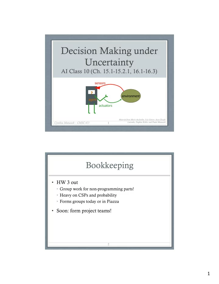
environment agent

?

sensors actuators

Bookkeeping

• HW 3 out
• Group work for non-programming parts!
• Heavy on CSPs and probability
• Forms groups today or in Piazza
• Soon: form project teams!

2

2

Today’s Class

• Making Decisions Under Uncertainty
• Tracking Uncertainty over Time
• Decision Making under Uncertainty
• Project groups, part 1 ß ?

3

Introduction

• The world is not a well-defined place.
• Sources of uncertainty
• Uncertain inputs: What’s the temperature?
• Uncertain (imprecise) definitions: Is Obama a good

president?

• Uncertain (unobserved) states: Where is the pit?
• There is uncertainty in inferences
• If I have a blistery, itchy rash and was gardening all

weekend I probably have poison ivy

4

3

Probabilistic reasoning only gives probabilistic results (summarizes uncertainty from various sources)

• Uncertain inputs
• Missing data
• Noisy data
• Uncertain knowledge
• >1 cause à >1 effect
• Incomplete knowledge of

causality

• Probabilistic effects
• Uncertain outputs
• Default reasoning (even

deduction) is uncertain

• Abduction & induction

inherently uncertain

• Incomplete deductive

inference can be uncertain

• Derived result is formally

correct, but wrong in real world

5

Sources of Uncertainty Reasoning Under Uncertainty

• People make successful decisions all the time

anyhow.

• How?
• More formally: how do we do reasoning under

uncertainty, with inexact knowledge?

• Step one: understanding what we know

6

4

MODELING UNCERTAINTY OVER TIME

7

States and Observations

• We don’t have a continuous view of world
• People don’t either!
• We see things as a series of snapshots
• Observations, associated with time slices
• t1, t2, t3, …
• Each snapshot contains all variables, observed or not
• Xt = (unobserved) state variables at time t; observation at t is Et
• This is world state at time t

8

5

environment agent

?

sensors actuators

t1, t2, t3, …

Temporal Probabilistic Agent

9

Time and Uncertainty

• The world changes
• Examples: diabetes management, traffic monitoring
• Tasks: track it; predict it
• Basic idea:
• Copy state and evidence variables for each time step
• Model uncertainty in change over time
• Incorporate new observations as they arrive

10

6

Time and Uncertainty

• Basic idea:
• Copy state and evidence variables for each time step
• Model uncertainty in change over time
• Incorporate new observations as they arrive
• Xt = unobservable state variables at time t:

BloodSugart, StomachContentst

• Et = evidence variables at time t:

MeasuredBloodSugart, PulseRatet, FoodEatent

• Assuming discrete time steps

11

States, Slightly More formally

• Process of change is viewed as series of snapshots
• Time slices
• Each describing the state of the world at a particular time
• Each time slice is represented by a set of random

variables indexed by t:

1. the set of unobservable state variables Xt 2. the set of observable evidence variables Et

• The observation at time t is Et = et for some set of

values et

• Xa:b denotes the set of variables from Xa to Xb

12

7

Transition and Sensor Models

• Transition model
• Models how the world changes over time
• Specifies a probability distribution
• Over state variables at time t
• Given values at previous times
• Sensor model
• Models how evidence gets its values (sensor data)
• E.g.: BloodSugart à MeasuredBloodSugart

P(Xt | X0:t-1)

How big can this get?

13

• Markov Assumption:
• Xt depends on some finite (usually fixed) number of previous Xi’s
• First-order Markov process: P(Xt|X0:t-1) = P(Xt|Xt-1)
• kth order: depends on previous k time steps
• Sensor Markov assumption: P(Et|X0:t, E0:t-1) = P(Et|Xt)
• Agent’s observations depend only on the actual current state of the

world

X

14

Markov Assumption

8

• Infinitely many possible values of t
• Does each timestep need a distribution?
• Assume stationary process:
• Changes in the world state are governed by laws that do

not themselves change over time

• Transition model P(Xt|Xt-1) and sensor model P(Et|Xt)

are time-invariant, i.e., they are the same for all t

15

Stationary Process

• Given:
• Transition model:

P(Xt|Xt-1)

• Sensor model:

P(Et|Xt)

• Prior probability:

P(X0)

• Then we can specify complete joint distribution
• f a sequence of states:

P(X0, X1,..., Xt, E1,..., Et) = P(X0) P(Xi | Xi−1)P(Ei | Xi)

i=1 t

∏

16

Complete Joint Distribution

9

Raint-1 Umbrellat-1 Raint Umbrellat Raint+1 Umbrellat+1

Rt-1 P(Rt|Rt-1) T F 0.7 0.3 Rt P(Ut | Rt) T F 0.9 0.2

This should look like a finite state automaton (since it is one)

17

Example

• Filtering or monitoring: P(Xt|e1,…,et)

Compute the current belief state, given all evidence to date

• Prediction: P(Xt+k|e1,…,et)

Compute the probability of a future state

• Smoothing: P(Xk|e1,…,et)

Compute the probability of a past state (hindsight)

• Most likely explanation:

arg maxx1,..xtP(x1,…,xt|e1,…,et) Given a sequence of observations, find the sequence of states that is most likely to have generated those observations

18

Inference Tasks

10

• Filtering: What is the probability that it is raining today,

given all of the umbrella observations up through today?

• Prediction: What is the probability that it will rain the day

after tomorrow, given all of the umbrella observations up through today?

• Smoothing: What is the probability that it rained yesterday,

given all of the umbrella observations through today?

• Most likely explanation: If the umbrella appeared the first

three days but not on the fourth, what is the most likely weather sequence to produce these umbrella sightings?

19

Examples

• Maintain a current state estimate and update it
• Rather than looking at all percepts (observed values) in history
• So, given result of filtering up to t, compute t+1 from et+1
• We use recursive estimation to compute

P(Xt+1 | e1:t+1) as a function of et+1 and P(Xt | e1:t)

• We can write this as:

P(Xt+1 | e1:t+1) = P(Xt+1 | e1:t,et+1)

20

Filtering

11

• P(Xt+1 | e1:t+1) as a function of et+1 and P(Xt | e1:t)
• This leads to a recursive definition:

f1:t+1 = α FORWARD (f1:t, et+1)

P(Xt+1 | e1:t+1) = P(Xt+1 | e1:t,et+1) =α P(et+1 | Xt+1,e1:t) P(Xt+1 | e1:t) =α P(et+1 | Xt+1) P(Xt+1 | e1:t) =α P(et+1 | Xt+1) P(Xt+1 | xt) P(xt | e1:t)

xt

∑

21

Filtering 2

Raint-1 Umbrellat-1 Raint Umbrellat Raint+1 Umbrellat+1

Rt-1 P(Rt|Rt-1) T F 0.7 0.3 Rt P(Ut|Rt) T F 0.9 0.2

What is the probability of rain on Day 2, given a uniform prior of rain

• n Day 0, U1 = true, and U2 = true?

P(Xt +1 |e1:t +1) = α P(et +1 | Xt +1) P(Xt +1 | Xt) P(Xt |e1:t)

X t

∑

22

Filtering Example

12

23

Decision Making Under Uncertainty

Decision Making Under Uncertainty

• Many environments have multiple possible
• utcomes
• Some of these outcomes may be good; others may

be bad

• Some may be very likely; others unlikely
• What’s a poor agent to do?

24

13

Reasoning Under Uncertainty

• So how do we do reasoning under uncertainty and

with inexact knowledge?

• Heuristics
• Mimic heuristic knowledge processing methods used by experts
• Empirical associations
• Experiential reasoning
• Based on limited observations
• Probabilities
• Objective (frequency counting)
• Subjective (human experience )

25

?

b a c {a,b,c} à decision that is best for worst case

?

b a c {a(pa), b(pb), c(pc)} à decision that maximizes expected utility value Non-deterministic model Probabilistic model ~ Adversarial search

26

Non-deterministic vs. Probabilistic Uncertainty

14

Decision Theory

• Combine probability and utility

à Agent that makes rational decisions

• On average, lead to desired outcome
• Immediate simplifications:
• Want most desirable immediate outcome (episodic)
• nondeterministic, partially observable world
• Definition: result of an action a leads to outcome s’:
• RESULT(a) is a random variable; domain is possible outcomes
• P(RESULT(a) = s’ | a, e)

27

Expected Utility

• Goal: find best expected outcome
• Random variable X with:
• n values x1,…,xn
• Distribution (p1,…,pn)
• X is the state reached after doing an action A

under uncertainty

• Utility function U(s) is the utility of a state, i.e.,

desirability

28

15

Expected Utility

• X is state reached after doing an action A under

uncertainty

• U(s) is the utility of a state ß desirability
• The expected utility of action A, given evidence

EU(a|e), is average utility of outcomes (states in S), weighted by probability an action occurs: EU[A] = Si=1,…,n p(xi|A)U(xi)

29

s0 s3 s2 s1

A1

0.2 0.7 0.1 100 50 70

U(A1, S0) = 100 x 0.2 + 50 x 0.7 + 70 x 0.1 = 20 + 35 + 7 = 62

One State/One Action Example

30

16

s0 s3 s2 s1

A1

0.2 0.7 0.1 100 50 70

A2

s4

0.2 0.8 80

• U (A1, S0) = 62
• U (A2, S0) = 74
• U (S0) = maxa{U(a,S0)}

= 74

One State/Two Actions Example

31

s0 s3 s2 s1

A1

0.2 0.7 0.1 100 50 70

A2

s4

0.2 0.8 80

• U (A1, S0) = 62 – 5 = 57
• U (A2, S0) = 74 – 25 = 49
• U (S0) = maxa{U(a, S0)}

= 57

• 5
• 25

Introducing Action Costs

32

17

MEU Principle

• A rational agent should choose the action that

maximizes agent’s expected utility

• This is the basis of the field of decision theory
• The MEU principle provides a normative criterion

for rational choice of action

• …AI is solved!

33

Not Quite…

• Must have a complete model of:
• Actions
• Utilities
• States
• Even if you have a complete model, decision making is

computationally intractable

• In fact, a truly rational agent takes into account the utility of

reasoning as well (bounded rationality)

• Nevertheless, great progress has been made in this area
• We are able to solve much more complex decision-theoretic problems

than ever before

34

18

Axioms of Utility Theory

• Orderability

(A>B) ∨ (A<B) ∨ (A~B)

• Transitivity
• (A>B) ∧ (B>C) ⇒ (A>C)
• Continuity
• A>B>C ⇒ ∃p [p,A; 1-p,C] ~ B
• Substitutability
• A~B ⇒ [p,A; 1-p,C]~[p,B; 1-p,C]
• Monotonicity
• A>B ⇒ (p≥q ⇔ [p,A; 1-p,B] >~ [q,A; 1-q,B])
• Decomposability
• [p,A; 1-p, [q,B; 1-q, C]] ~ [p,A; (1-p)q, B; (1-p)(1-q), C]

35

Money Versus Utility

• Money <> Utility
• More money is better, but not always in a linear

relationship to the amount of money

• Expected Monetary Value
• Risk-averse: U(L) < U(SEMV(L))
• Risk-seeking: U(L) > U(SEMV(L))
• Risk-neutral: U(L) = U(SEMV(L))

36

19

Value Function

• Provides a ranking of alternatives, but not a

meaningful metric scale

• Also known as an “ordinal utility function”
• Sometimes, only relative judgments (value

functions) are necessary

• At other times, absolute judgments (utility

functions) are required

37