
SLIDE 1
1
Data Mining Techniques: Cluster Analysis
Mirek Riedewald Many slides based on presentations by Han/Kamber, Tan/Steinbach/Kumar, and Andrew Moore
Cluster Analysis Overview
- Introduction
- Foundations: Measuring Distance (Similarity)
- Partitioning Methods: K-Means
- Hierarchical Methods
- Density-Based Methods
- Clustering High-Dimensional Data
- Cluster Evaluation
2
What is Cluster Analysis?
- Cluster: a collection of data objects
– Similar to one another within the same cluster – Dissimilar to the objects in other clusters
- Unsupervised learning: usually no training set
with known “classes”
- Typical applications
– As a stand-alone tool to get insight into data properties – As a preprocessing step for other algorithms
3
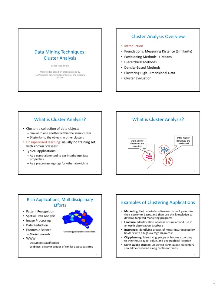
What is Cluster Analysis?
4
Inter-cluster distances are maximized Intra-cluster distances are minimized
Rich Applications, Multidisciplinary Efforts
- Pattern Recognition
- Spatial Data Analysis
- Image Processing
- Data Reduction
- Economic Science
– Market research
- WWW
– Document classification – Weblogs: discover groups of similar access patterns
5
Clustering precipitation in Australia
Examples of Clustering Applications
- Marketing: Help marketers discover distinct groups in
their customer bases, and then use this knowledge to develop targeted marketing programs
- Land use: Identification of areas of similar land use in
an earth observation database
- Insurance: Identifying groups of motor insurance policy
holders with a high average claim cost
- City-planning: Identifying groups of houses according
to their house type, value, and geographical location
- Earth-quake studies: Observed earth quake epicenters
should be clustered along continent faults
6