
SLIDE 1
CS234 Notes - Lecture 14 Model Based RL, Monte-Carlo Tree Search
Anchit Gupta, Emma Brunskill June 14, 2018
1 Introduction
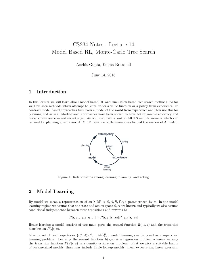
In this lecture we will learn about model based RL and simulation based tree search methods. So far we have seen methods which attempt to learn either a value function or a policy from experience. In contrast model based approaches first learn a model of the world from experience and then use this for planning and acting. Model-based approaches have been shown to have better sample efficiency and faster convergence in certain settings. We will also have a look at MCTS and its variants which can be used for planning given a model. MCTS was one of the main ideas behind the success of AlphaGo. Figure 1: Relationships among learning, planning, and acting
2 Model Learning
By model we mean a representation of an MDP < S, A, R, T, γ> parametrized by η. In the model learning regime we assume that the state and action space S, A are known and typically we also assume conditional independence between state transitions and rewards i.e P[st+1, rt+1|st, at] = P[st+1|st, at]P[rt+1|st, at] Hence learning a model consists of two main parts the reward function R(.|s, a) and the transition distribution P(.|s, a). Given a set of real trajectories {Sk
t , Ak t Rk t , ..., Sk T }K k=1 model learning can be posed as a supervised
learning problem. Learning the reward function R(s, a) is a regression problem whereas learning the transition function P(s′|s, a) is a density estimation problem. First we pick a suitable family
- f parametrized models, these may include Table lookup models, linear expectation, linear gaussian,