Convex Hull Algorithms 2D Basic facts Algorithms: Nave, Gift - PDF document

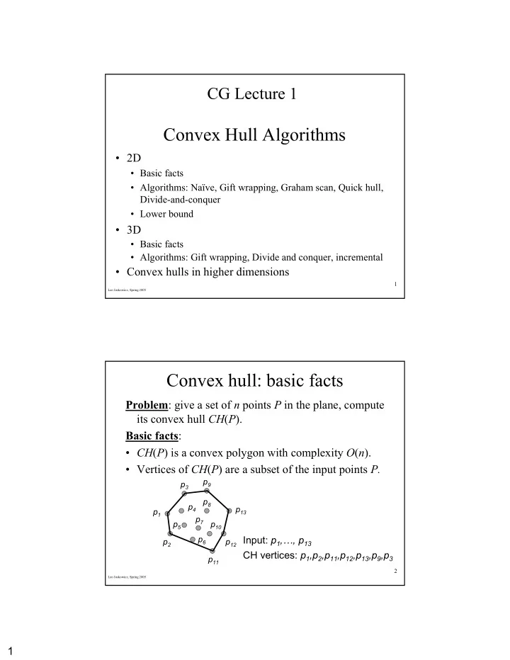
CG Lecture 1 CG Lecture 1 Convex Hull Algorithms • 2D • Basic facts • Algorithms: Naïve, Gift wrapping, Graham scan, Quick hull, Divide-and-conquer • Lower bound • 3D • Basic facts • Algorithms: Gift wrapping, Divide and conquer, incremental • Convex hulls in higher dimensions 1 Leo Joskowicz, Spring 2005 Leo Joskowicz, Spring 2005 Convex hull: basic facts Convex hull: basic facts Problem : give a set of n points P in the plane, compute its convex hull CH ( P ). Basic facts : • CH ( P ) is a convex polygon with complexity O ( n ). • Vertices of CH ( P ) are a subset of the input points P. p 9 p 3 p 8 p 4 p 13 p 1 p 7 p 5 p 10 p 6 Input: p 1 ,…, p 13 Input: p 2 p 12 CH vertices: p 1 ,p 2 ,p 11 ,p 12 ,p 13 ,p 9 ,p 3 CH vertices: p 11 2 Leo Joskowicz, Spring 2005 Leo Joskowicz, Spring 2005 1

Naive algorithm Naive algorithm Algorithm • For each pair of points construct its connecting segment and supporting line . • Find all the segments whose supporting Yes Yes lines divide the plane into two halves, such that one half plane contains all the other points. • Construct the convex hull out of these No No segments. Time complexity • All pairs: ⎛ ⎞ n − n n ( 1) = = 2 O ( ) O ( ) O n ( ) ⎜ ⎟ 2 2 ⎝ ⎠ • Check all points for each pair: O ( n ) each, O ( n 3 ) total. 3 Leo Joskowicz, Spring 2005 Leo Joskowicz, Spring 2005 Triangle Area Triangle Area ⋅ = − × − 2 Area ( P P ) ( P P ) 2 1 3 1 = − ⋅ − α P P P P sin 2 1 3 1 P 3 (x 3 ,y 3 ) − − x x y y = 2 1 2 1 − − x x y y 3 1 3 1 α x y 1 1 1 P 1 (x 1 ,y 1 ) P 2 (x 2 ,y 2 ) = x y 1 2 2 x y 1 3 3 The determinant is twice the area of the triangle whose vertices are the rows of the matrix. 4 Leo Joskowicz, Spring 2005 Leo Joskowicz, Spring 2005 2

Orientation and point classification Orientation and point classification ( x 1 , y 1 ) x y 1 1 1 1 = Area x y 1 2 2 2 + x y 1 3 3 ( x 2 , y 2 ) ( x 3 , y 3 ) • The area sign indicates the orientation of the points. • Positive area ≡ counterclockwise orientation ≡ left turn. • Negative area ≡ clockwise orientation ≡ right turn. • This test can be used to determine whether a given point is “above” or “below” a given line 5 Leo Joskowicz, Spring 2005 Leo Joskowicz, Spring 2005 Triangle Area Triangle Area ⋅ = − × − 2 Area ( P P ) ( P P ) 2 1 3 1 = − ⋅ − α P P P P sin 2 1 3 1 P 3 (x 3 ,y 3 ) − − x x y y = 2 1 2 1 − − x x y y 3 1 3 1 α x y 1 1 1 P 1 (x 1 ,y 1 ) P 2 (x 2 ,y 2 ) = x y 1 2 2 x y 1 3 3 The determinant is twice the area of the triangle whose vertices are the rows of the matrix. 6 Leo Joskowicz, Spring 2005 Leo Joskowicz, Spring 2005 3

Orientation and point classification Orientation and point classification ( x 1 , y 1 ) x y 1 1 1 1 = Area x y 1 2 2 2 + x y 1 3 3 ( x 2 , y 2 ) ( x 3 , y 3 ) • The area sign indicates the orientation of the points. • Positive area ≡ counterclockwise orientation ≡ left turn. • Negative area ≡ clockwise orientation ≡ right turn. • This test can be used to determine whether a given point is “above” or “below” a given line 7 Leo Joskowicz, Spring 2005 Leo Joskowicz, Spring 2005 Possible problems Possible problems • Degenerate cases, e.g., 3 collinear points, may harm the correctness of the algorithm. Segments AB , BC and A AC will all be included in the B convex hull. C • Numerical problems – We might conclude that none of the three segments (or a wrong pair of them) belongs to the convex hull. • Question: How is colinearity detected? 8 Leo Joskowicz, Spring 2005 Leo Joskowicz, Spring 2005 4

General position assumption General position assumption • When designing a geometric algorithm, we first make some simplifying assumptions, e.g.: • No three collinear points; • No two points with the same x or y coordinate; • Other configurations: no three points on a circle, … • Later, we consider the general case: • Behavior of algorithm to degenerate cases? • Will the correctness be preserved? • Will the running time remain the same? • Modify/extend algorithm to handle degeneracies 9 Leo Joskowicz, Spring 2005 Leo Joskowicz, Spring 2005 Gift wrapping algorithm Gift wrapping algorithm p 3 Algorithm: p 8 p 13 1. Find the lowest point p 1 and its hull edge e p 4 p 1 2. For each remaining point p i ( i > 2) do p 7 p 5 p 10 • Compute the CCW angle α i from the p 6 p 2 p 2 previous hull edge • Let p j be the point with the smallest α i p 1 • Make ( p 1 p i ) the new hull edge Rotate counterclockwise a line through p 1 until it touches one of the other points Time complexity: O ( n 2 ) In fact, the complexity is O( nh ), where n is the input size and h is the hull size. 10 Leo Joskowicz, Spring 2005 Leo Joskowicz, Spring 2005 5

Line equation and angle Line equation and angle • Let ( x 1 ,y 1 ) and ( x 2 ,y 2 ) be two points. • The explicit line equation is: = + y mx c − − y y y x y x y = mx+c y = mx+c = + y 2 1 x 1 2 2 1 − − x x x x m = tan m = tan θ θ 2 1 2 1 − y y θ = tan 2 1 c c − x x 2 1 • Singularity at x 1 = x 2 (vertical line) 11 Leo Joskowicz, Spring 2005 Leo Joskowicz, Spring 2005 Graham’ ’s scan algorithm s scan algorithm Graham Algorithm: • Find a point p 0 in the interior of the hull. • Compute the CCW angle α i from p 0 to all p 0 other points. • Sort the points by angle α i. • Construct the boundary by scanning the points in the sorted order and performing only “right turns” (trim off “left turns”). p 0 p 0 Use a stack to process sorted points Time Complexity : O ( n log n ) Right turn Left turn Right turn Left turn Question: How do we check for a right or left turn? 12 Leo Joskowicz, Spring 2005 Leo Joskowicz, Spring 2005 6

Graham’ ’s s scan: complexity analysis Graham scan: complexity analysis • Sorting – O( n log n ) • D i = number of points popped on processing p i , n n ∑ ∑ = + = + time ( D 1) n D i i = = i 1 i 1 • Each point is pushed on the stack only once. • Once a point is popped – it cannot be popped again. • Hence n ∑ ≤ D n i = i 1 13 Leo Joskowicz, Spring 2005 Leo Joskowicz, Spring 2005 Quick hull algorithm Quick hull algorithm a Algorithm : • Find four extreme points of P: highest a , lowest c b , leftmost c , rightmost d. d • Discard all points in the quadrilateral interior • Find the hulls of the four triangular regions exterior to the quadrilateral. b • To process triangular regions, find the extreme point in linear time. Two new exterior regions A, B will be formed, each processed separately. • Recurse until no points are left in the exterior: the convex hull is the union of the exteriors. extreme point c Time Complexity: |B|= β |B|= |A|= α α |A|= T ( n ) = O ( n )+ T ( α )+ T ( β ) where α + β =n– 1 a = T ( n –1) + O ( n ) = O ( n 2 ) worst case! 14 b Leo Joskowicz, Spring 2005 Leo Joskowicz, Spring 2005 7

Divide- -and and- -Conquer Conquer Divide Algorithm: median median • Find a point with a median x coordinate in O ( n ) time tangents tangents • Partition point set in two halves • Compute the convex hull of each half (recursive execution) • Combine the two convex hulls by finding their upper and lower tangents in O ( n ). left hull left hull right hull right hull Time Complexity: O ( n log n ) ⎛ ⎞ n = + T ( n ) 2 T ⎜ ⎟ O ( n ) ⎝ 2 ⎠ 15 Leo Joskowicz, Spring 2005 Leo Joskowicz, Spring 2005 Finding tangents (1) Finding tangents (1) • Two disjoint convex polygons have four tangents that classify them as either being entirely to the left (+) or to the right ( − ) of the line: (+,+) (+,+) (+, − (+, − ) ) ( − ( − ,+) ,+) ( − ( − , , − − ) ) 16 Leo Joskowicz, Spring 2005 Leo Joskowicz, Spring 2005 8

Finding tangents (2) Finding tangents (2) Lower tangent: Connect rightmost 1: (- -,+) ,+) 1: ( point of left hull to 2: (- -,*) ,*) 2: ( leftmost point in right hull and 5: (*,- -) ) 5: (*, 3: (*,*) 3: (*,*) “walk” around both boundaries until the lower tangent is reached. Complexity : O ( n ) . 17 Leo Joskowicz, Spring 2005 Leo Joskowicz, Spring 2005 Lower bound for convex hull in 2D Lower bound for convex hull in 2D Claim: Convex hull computation takes Θ ( n log n ) Proof: reduction from Sorting to Convex Hull: • Given n real values x i , generate n points on the graph of a convex function, e.g. ( x i ,x i 2 ). • Compute the (ordered) convex Complexity(CH)= Ω ( n log n ) hull of the points. Since there is a O( n log n )-time algorithm, • The order of the convex hull Complexity(CH)= Θ ( n log n ) points is the order of the x i . 18 Leo Joskowicz, Spring 2005 Leo Joskowicz, Spring 2005 9