SLIDE 1 1
ECO 300 – Fall 2005 – October 11
CONSUMER BEHAVIOR UNDER UNCERTAINTY – PART 2 SOME PROBLEMS WITH EXPECTED UTILITY APPROACH (P-R pp. 180-3)
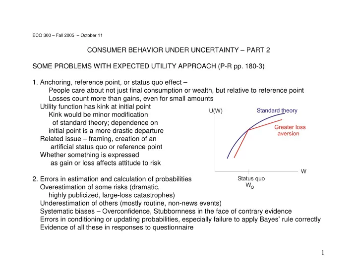
- 1. Anchoring, reference point, or status quo effect –
People care about not just final consumption or wealth, but relative to reference point Losses count more than gains, even for small amounts Utility function has kink at initial point Kink would be minor modification
- f standard theory; dependence on
initial point is a more drastic departure Related issue – framing, creation of an artificial status quo or reference point Whether something is expressed as gain or loss affects attitude to risk
- 2. Errors in estimation and calculation of probabilities
Overestimation of some risks (dramatic, highly publicized, large-loss catastrophes) Underestimation of others (mostly routine, non-news events) Systematic biases – Overconfidence, Stubbornness in the face of contrary evidence Errors in conditioning or updating probabilities, especially failure to apply Bayes’ rule correctly Evidence of all these in responses to questionnaire
SLIDE 2 2
Consider your responses to Questions 4 and 5 in the questionnaire If you are an expected utility maximizer with utility function U, then your expected utilities from the various random prospects are A: 0.33 U(2500) + 0.66 U(2400) + 0.01 U(0) B: U(2400) C: 0.33 U(2500) + 0.67 U(0) D: 0.34 U(2400) + 0.66 U(0) You prefer A to B if and only if 0.33 U(2500) + 0.66 U(2400) + 0.01 U(0) > U(2400),
- r 0.33 U(2500) + 0.01 U(0) > 0.34 U(2400)
You prefer C to D if and only if 0.33 U(2500) + 0.67 U(0) > 0.34 U(2400) + 0.66 U(0)
- r 0.33 U(2500) + 0.01 U(0) > 0.34 U(2400)
Therefore you should prefer A to B if and only if you prefer C to D Choice such as B in Question 4 and C in Question 5 is just plain inconsistent with expected utility maximization regardless of attitude to risk – whether U is concave or convex But many people make just such choice – as 20 out of 34 responders in this class! Some having seen this calculation may change their mind; others won’t Nothing irrational about such behavior, it can have underlying complete, transitive preferences But cannot be expressed as expected utility maximization
SLIDE 3
3 ALTERNATIVES TO EXPECTED UTILITY Prospect Theory of Kahneman and Tversky – Decision process consists of two phases: (1) Editing phase that organizes, reformulates, and simplifies options This is where status quo and framing effects originate (2) Evaluation phase. This uses not only a utility scale for prospects, U(x), but also a weighting scale for probabilities, B(p) Overall objective function: if there are n “edited prospects” Maximize B(p1) U(x1) + B(p2) U(x2) + ... + B(pn) U(xn) Typically, B(p) > p for small p, B(p) < p for p close to 1, and B(p1) + B(p2) + ... + B(pn) < 1 Minimax regret – Consider the outcomes (wealth, or utility): Scenario 1 2 Action 1 a b 2 c d Suppose a > c, and d > b, so action 1 is better in scenario 1 and action 2 in scenario 2 If you do 1 and scenario 2 materializes, you get b instead of d; define “regret” of action 1 as (d-b) Similarly regret of action 2 is (a-c). Rule - Choose the action with the smaller regret Merit - Don’t need probabilities. Defect - May be guarding against highly unlikely events. Each of these has its own difficulties – such a person is subject to a “Dutch book”, will accept a succession of bets in a cycle that will make expected loss
SLIDE 4 4 INSURANCE (brief treatment in P-R pp. 166-8) Consider a consumer with the initial wealth of W0 = $10 million Faces 10% risk that half of this would be wiped out (big house in Stanford destroyed by earthquake or one in Palm Beach by hurricane) Can buy insurance at price p per dollar of coverage. If buys x dollars, pays px right now, and gets back x if suffers loss So faces risky prospect: 10% probability final wealth W1 = 10 - 5 + x - p x = 5 + (1-p) x 90% probability final wealth W2 = 10 - p x Utility function is U(W) = ln(W) Expected utility is EU = 0.1 * ln[W1] + 0.9 * ln[W2] = 0.1 * ln[5 + (1-p) x] + 0.9 * ln[10-p x] Chooses x to maximize this. Two methods: MAT 103 method: Use the “chain rule” for differentiation of a function of a function dEU
dx W dW dx W dW dx p p x p px = + = − + − + − − 01 1 0 9 1 01 1 5 1 09 10
1 1 2 2
. . . ( ) ( ) .
Set this equal to zero, and simplify:
01 1 10 0 9 5 1 . ( ) ( ) . [ ( ) ] − − − + − = p px p p x
SLIDE 5 5
x p p p = − − 1 55 1 . ( )
This is the demand curve for insurance. See figure. Observe p = 0.1 is “actuarially fair insurance”, and at this price, x = 5 : full coverage demanded Typically, p > 0.1 because of insurance company’s admin. costs and market power So consumer chooses partial coverage Other reason for partial coverage - moral hazard Mathematically, could contemplate p < 0.1, but this is economically irrelevant: insurance co. offering this would lose money; moral hazard would be overwhelming When p = 0.18, x = 0 If insurance is sufficiently “unfairly priced” even risk-averse consumer will prefer to bear the whole risk
SLIDE 6
6 ALTERNATIVE INTERPRETATION OF INSURANCE – MARKETS FOR RISK (not in P-R) When you pay say p = 0.12 for a dollar of fire insurance on your house you are “betting” 0.12; you “win the bet” and get $1-0.12 = 0.88 if the fire occurs, you “lose the bet” and lose 0.12 if the fire does not occur. More generally, consider a market in “contingent claims” held before anyone knows which of the events 1 and 2 occurs The objects traded in this market are “betting slips” You buy and sell these ahead of time. Then, after the uncertainty is resolved you cash in the slips corresponding to the event that occurs; the other kind are worthless after the fact A scenario-1 betting slip will pay $1 if scenario 1 occurs, 0 otherwise A scenario-2 betting slip will pay $1 if scenario 2 occurs, 0 otherwise The market determines the prices say p(1), p(2) of these slips; the demand and supply depend on probabilities and participants’ risk attitudes If you hold one of each kind of slip, you will get $1 for sure; so prices p(1) + p(2) = 1 If time to resolution of uncertainty is distant, sum = 1/(1+interest rate) In real world there are zillions of different scenarios, and zillions of assets can be created by bundling and rebundling the “betting slips” for them
SLIDE 7
7 Financial markets trade in objects of exactly this kind, usually bundled in particular ways Equity stocks give you different dividends and capital gains (or losses) in different scenarios corresponding to how well or poorly the firm does Bonds give interest and capital gains or losses as interest rates change Options, derivatives are ways of rebundling risks to suit specific classes of investors Other examples: [1] Contingent claims markets on weather scenarios (temperature on particular day / season) These are used by energy producers and utilities to hedge their costs Website http://www.evomarkets.com/weather/ [2] Political betting markets on elections - http://www.biz.uiowa.edu/iem/ [3] Mortgage-backed securities and collateralized mortgage obligations Website http://www.investopedia.com/terms/m/mbs.asp Bad news – to be a real expert in such securities, to be actually able to design new ones, and make seven-figure incomes, requires very high-end math: MAT 315 real analysis, MAT 391 stochastic processes etc.
SLIDE 8
8 EFFICIENT ALLOCATION OF RISK (not in P-R) Can markets greatly reduce or eliminate risk for all participants? Sometimes yes: [1] negative correlation enables elimination by sharing [2] law of large numbers allows substantial reduction by pooling independent risks But more generally, risks can only be traded – for every hedger there is a speculator on the other side of the trade Then the question is whether markets will achieve efficient allocation of risks Some such tendencies can be identified – less risk-averse person will accept the risk for a smaller price than what a more risk-averse person is willing to pay So mutually beneficial trade – risk ends up with whoever is most willing to bear it But problems arise, mainly because of asymmetric information Moral hazard – One person’s actions can affect probability or magnitude of risk But others cannot observe this, so cannot write contract to exclude such actions Then e.g. availability of insurance may make the insured behave carelessly To cope with this: only partial insurance is offered Adverse selection – One person knows more about the nature of the risk than another To cope with this: strategies of signaling and screening Example: Potential employers want quantitative skills, dedication, perseverance, ... You can signal these qualities by taking tough courses, sticking to them, getting good grades Or employer can screen applicants by requiring such courses and grades on your resume In either case - the action must be such that someone who does not have the desired characteristic would find it too costly to imitate the action