Constraint satisfaction problems (CSPs) Standard search problem: - PowerPoint PPT Presentation

Constraint satisfaction problems (CSPs) Standard search problem: state is a “black box”—any old data structure that supports goal test, eval, successor Constraint Satisfaction Problems CSP: state is defined by variables X i with values from domain D i goal test is a set of constraints specifying Chapter 6 allowable combinations of values for subsets of variables Simple example of a formal representation language Allows useful general-purpose algorithms with more power than standard search algorithms Chapter 6 1 Chapter 6 3 Outline 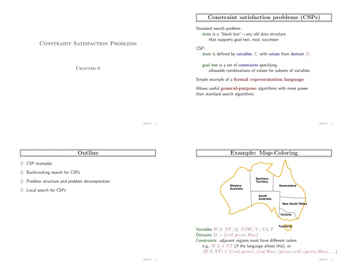Example: Map-Coloring ♦ CSP examples ♦ Backtracking search for CSPs Northern ♦ Problem structure and problem decomposition Territory Western Queensland Australia ♦ Local search for CSPs South Australia New South Wales Victoria Tasmania Variables WA , NT , Q , NSW , V , SA , T Domains D i = { red, green, blue } Constraints: adjacent regions must have different colors e.g., WA � = NT (if the language allows this), or ( WA, NT ) ∈ { ( red, green ) , ( red, blue ) , ( green, red ) , ( green, blue ) , . . . } Chapter 6 2 Chapter 6 4

Example: Map-Coloring contd. Varieties of CSPs Discrete variables O ( d n ) complete assignments finite domains; size d ⇒ ♦ e.g., Boolean CSPs, incl. Boolean satisfiability (NP-complete) infinite domains (integers, strings, etc.) Northern Territory ♦ e.g., job scheduling, variables are start/end days for each job Western Queensland Australia ♦ need a constraint language, e.g., StartJob 1 + 5 ≤ StartJob 3 ♦ linear constraints solvable, nonlinear undecidable South Australia New South Wales Continuous variables ♦ e.g., start/end times for Hubble Telescope observations Victoria ♦ linear constraints solvable in poly time by LP methods Tasmania Solutions are assignments satisfying all constraints, e.g., { WA = red, NT = green, Q = red, NSW = green, V = red, SA = blue, T = green } Chapter 6 5 Chapter 6 7 Constraint graph Varieties of constraints Unary constraints involve a single variable, Binary CSP: each constraint relates at most two variables e.g., SA � = green Constraint graph: nodes are variables, arcs show constraints Binary constraints involve pairs of variables, e.g., SA � = WA NT Q Higher-order constraints involve 3 or more variables, WA e.g., cryptarithmetic column constraints SA NSW Preferences (soft constraints), e.g., red is better than green often representable by a cost for each variable assignment V → constrained optimization problems Victoria T General-purpose CSP algorithms use the graph structure to speed up search. E.g., Tasmania is an independent subproblem! Chapter 6 6 Chapter 6 8

Example: Cryptarithmetic Standard search formulation (incremental) Let’s start with the straightforward, dumb approach, then fix it States are defined by the values assigned so far T W O O F T U W R + T W O ♦ Initial state: the empty assignment, { } F O U R ♦ Successor function: assign a value to an unassigned variable that does not conflict with current assignment. X 3 X 2 X 1 ⇒ fail if no legal assignments (not fixable!) ♦ Goal test: the current assignment is complete Variables: F T U W R O X 1 X 2 X 3 Domains: { 0 , 1 , 2 , 3 , 4 , 5 , 6 , 7 , 8 , 9 } Constraints 1) This is the same for all CSPs! alldiff ( F, T, U, W, R, O ) 2) Every solution appears at depth n with n variables ( d values each) O + O = R + 10 · X 1 , etc. ⇒ use depth-first search 3) Path is irrelevant, so can also use complete-state formulation 4) b = ( n − ℓ ) d at depth ℓ , hence n ! d n leaves!!!! Chapter 6 9 Chapter 6 11 Real-world CSPs Backtracking search Assignment problems Variable assignments are commutative, i.e., e.g., who teaches what class, who flies which flight [ WA = red then NT = green ] same as [ NT = green then WA = red ] Timetabling problems Order of the variable assignments is not important, pick an arbitrary order e.g., which class is offered when and where, which flight is scheduled Consider assignments to a different variable at each level (according to the when and where order) b = d and there are d n leaves Hardware configuration ⇒ Spreadsheets Depth-first search for CSPs with single-variable assignments Transportation scheduling is called backtracking search Factory scheduling Backtracking search is the basic uninformed algorithm for CSPs Floorplanning Can solve n -queens for n ≈ 25 Notice that many real-world problems involve real-valued variables Chapter 6 10 Chapter 6 12

Backtracking search Backtracking example function Backtracking-Search ( csp ) returns solution/failure return Recursive-Backtracking ( { } , csp ) function Recursive-Backtracking ( assignment , csp ) returns soln/failure if assignment is complete then return assignment var ← Select-Unassigned-Variable ( Variables [ csp ], assignment , csp ) for each value in Order-Domain-Values ( var , assignment , csp ) do if value is consistent with assignment given Constraints [ csp ] then add { var = value } to assignment result ← Recursive-Backtracking ( assignment , csp ) if result � = failure then return result remove { var = value } from assignment return failure Chapter 6 13 Chapter 6 15 Backtracking example Backtracking example Chapter 6 14 Chapter 6 16

Backtracking example Choosing a variable: Minimum remaining values Minimum remaining values (MRV): choose the variable with the fewest legal values Northern Territory Western Queensland Australia South Australia New South Wales Victoria Tasmania Chapter 6 17 Chapter 6 19 Improving backtracking efficiency Choosing a variable: Degree heuristic General-purpose methods can give huge gains in speed: Tie-breaker among MRV variables Degree heuristic: 1. Which variable should be assigned next? choose the variable with the most constraints on remaining variables 2. In what order should its values be tried? (highest degree) 3. Can we detect inevitable failure early? 4. Can we take advantage of problem structure? Northern Territory Western Queensland Australia South Australia New South Wales Victoria Tasmania Chapter 6 18 Chapter 6 20

Choosing a value: Least constraining value Forward checking (1-step look ahead) Given a variable, choose the least constraining value: • Keep track of remaining legal values for unassigned variables the one that rules out the fewest values in the remaining variables – Help MRV Allows 1 value for SA – Terminate search when any variable has no legal values Allows 0 values for SA WA NT Q NSW V SA T Northern Territory Western Queensland Australia South Australia New South Wales Victoria Tasmania Combining these heuristics (most-constraining variables, least-contraining values) makes 1000 queens feasible Chapter 6 21 Chapter 6 23 Forward checking (1-step look ahead) Forward checking (1-step look ahead) • Keep track of remaining legal values for unassigned variables • Keep track of remaining legal values for unassigned variables – Help MRV – Help MRV – Terminate search when any variable has no legal values – Terminate search when any variable has no legal values WA NT Q NSW V SA T WA NT Q NSW V SA T Northern Territory Western Queensland Australia South Australia New South Wales Victoria Tasmania Chapter 6 22 Chapter 6 24

Forward checking (1-step look ahead) Arc consistency (multi-step look ahead) Simplest form of propagation makes each arc consistent • Keep track of remaining legal values for unassigned variables X → Y is consistent iff – Help MRV for every value x of X there is some allowed y – Terminate search when any variable has no legal values WA NT Q NSW V SA T WA NT Q NSW V SA T Northern Territory Western Queensland Australia South Australia New South Wales Victoria Tasmania Chapter 6 25 Chapter 6 27 Constraint propagation Arc consistency (multi-step look ahead) Forward checking propagates information from assigned to unassigned vari- Simplest form of propagation makes each arc consistent ables, but doesn’t provide early detection for all failures: X → Y is consistent iff for every value x of X there is some allowed y WA NT Q NSW V SA T WA NT Q NSW V SA T NT and SA cannot both be blue! Northern Constraint propagation repeatedly enforces constraints locally Territory Western Queensland Australia South Australia New South Wales Victoria Tasmania Chapter 6 26 Chapter 6 28