SLIDE 1
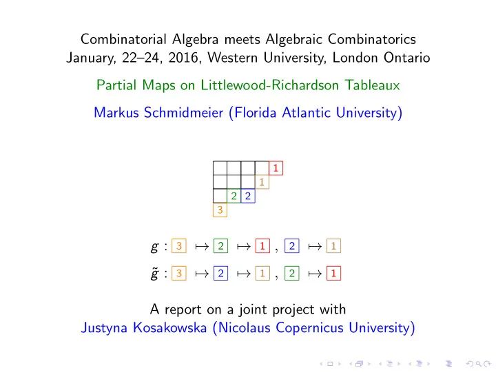
Combinatorial Algebra meets Algebraic Combinatorics January, 22–24, 2016, Western University, London Ontario Partial Maps on Littlewood-Richardson Tableaux Markus Schmidmeier (Florida Atlantic University)
3 2 2 1 1
g : 3 → 2 → 1 ,
2
→ 1 ˜ g : 3 → 2 → 1 ,
2
→ 1 A report on a joint project with Justyna Kosakowska (Nicolaus Copernicus University)
SLIDE 2
Littlewood-Richardson tableaux LR-coefficients and LR-tableaux in algebra The Green-Klein Theorem for embeddings Klein tableaux The lattice permutation property revisited Classifying embeddings with a p2-bounded submodule Partial maps Poles: Embeddings with a cyclic submodule Classifying direct sums of poles Tableaux which are horizontal and vertical strips Summary
SLIDE 3
- I. Littlewood-Richardson tableaux
Definition: An LR-tableau of shape (α, β, γ) is a Young diagram of shape β in which the region β \ γ contains α′
1 entries 1 , ..., α′ s entries s ,
where s = α1 is the length of α′, such that
◮ in each row, the entries are weakly increasing, ◮ in each column, the entries are strictly increasing, ◮ the lattice permutation property holds: For each ℓ > 1 and
each column c: on the right hand side of c, the number of entries ℓ − 1 is at least the number of entries ℓ.
SLIDE 4
- I. Littlewood-Richardson tableaux
Definition: An LR-tableau of shape (α, β, γ) is a Young diagram of shape β in which the region β \ γ contains α′
1 entries 1 , ..., α′ s entries s ,
where s = α1 is the length of α′, such that
◮ in each row, the entries are weakly increasing, ◮ in each column, the entries are strictly increasing, ◮ the lattice permutation property holds: For each ℓ > 1 and
each column c: on the right hand side of c, the number of entries ℓ − 1 is at least the number of entries ℓ. Example:
1 2 3 1 2 1 4 2 3 1
SLIDE 5
- I. Littlewood-Richardson tableaux
Definition: An LR-tableau of shape (α, β, γ) is a Young diagram of shape β in which the region β \ γ contains α′
1 entries 1 , ..., α′ s entries s ,
where s = α1 is the length of α′, such that
◮ in each row, the entries are weakly increasing, ◮ in each column, the entries are strictly increasing, ◮ the lattice permutation property holds: For each ℓ > 1 and
each column c: on the right hand side of c, the number of entries ℓ − 1 is at least the number of entries ℓ. Example:
1 2 3 1 2 1 4 2 3 1
c = 2, ℓ = 2 : #{ 1 ′s} ≥ #{ 2 ′s}
SLIDE 6 LR-coefficients in algebra
LR-tableaux occur in many exciting situations in algebra, but on the surface it appears that only their number is needed: The LR-coefficient cβ
α,γ counts the number of LR-tableaux of
shape (α, β, γ).
◮ Symmetric functions: Product of Schur polynomials
sα · sγ =
β cβ α,γ sβ ◮ Horn’s Problem: There are Hermetian matrices A, B, C with
eigenvalues α, β, γ and A + C = B if and only if cβ
α,γ = 0 ◮ Green-Klein Theorem: There is a short exact sequence of
finite abelian p-groups (or of nilpotent linear operators) 0 → Nα → Nβ → Nγ → 0 if and only if cβ
α,γ = 0
Recall: Nα =
s
Z/(pαi)
Nα =
s
k[T]/(T αi) if α = (α1, . . . , αs)
SLIDE 7 The tableau of an embedding
Let 0 → Nα
f
→ Nβ → Nγ → 0 be a short exact sequence. Often we will just consider the monomorphism f : Nα → Nβ, or the embedding (A ⊂ B) where A = Imf and B = Nβ. Suppose in an embedding (A ⊂ B), the module A has Loewy length r (so r is minimal with prA = 0). Consider the modules B/A, B/pA, . . . , B/prA = B and their corresponding partitions γ = γ0, γ1, . . . , γr = β. Definition: The tableau of the embedding (A ⊂ B) is given by the Young diagram β where in each skew diagram γi \ γi−1 the boxes are labelled by
i .
Example: For the embedding ((p2, p, 1)) ⊂
Z (p6) ⊕ Z (p4) ⊕ Z (p),
the above modules have partitions (5, 2), (5, 2, 1), (5, 3, 1), (5, 4, 1), (6, 4, 1). P :
Γ :
4 3 2 1
SLIDE 8
The Green-Klein Theorem revisited
Hence the Green-Klein Theorem really is the following statement: Theorem (Green, Klein): Let α, β, γ be partitions.
◮ If 0 → Nα → Nβ → Nγ → 0 is a short exact sequence with
tableau Γ, then Γ is a Littlewood-Richardson tableau of shape (α, β, γ).
◮ Conversely, for each Littlewood-Richardson tableau Γ of shape
(α, β, γ), there exists a short exact sequence 0 → Nα → Nβ → Nγ → 0 with tableau Γ. For abelian p-groups, the Hall polynomial counts the embeddings corresponding to Γ, it is a monic polynomial of degree nβ − nα − nγ. For k-linear operators, k an algebraically closed field, the set of embeddings f : Nα → Nβ with cokernel Nγ forms a variety, with irreducible components indexed by the LR-tableaux.
SLIDE 9
- II. The lattice permutation property revisited
Recall that the lattice permutation property (LPP) states that in the LR-tableau Γ, for each ℓ > 1 and each column c: on the right hand side of c, the number of entries ℓ − 1 is at least the number
Example:
1 2 3 1 2 1 4 2 3 1
c = 2, ℓ = 2 : #{ 1 ′s} ≥ #{ 2 ′s}
SLIDE 10
- II. The lattice permutation property revisited
Recall that the lattice permutation property (LPP) states that in the LR-tableau Γ, for each ℓ > 1 and each column c: on the right hand side of c, the number of entries ℓ − 1 is at least the number
Example:
1 2 3 1 2 1 4 2 3 1
c = 2, ℓ = 2 : #{ 1 ′s} ≥ #{ 2 ′s} Equivalent to (LPP): For each ℓ > 1 and each row r > 1: the number of entries ℓ − 1 in row r − 1 or above is at least the number of entries ℓ in row r or above.
SLIDE 11
- II. The lattice permutation property revisited
Recall that the lattice permutation property (LPP) states that in the LR-tableau Γ, for each ℓ > 1 and each column c: on the right hand side of c, the number of entries ℓ − 1 is at least the number
Example:
1 2 3 1 2 1 4 2 3 1
c = 2, ℓ = 2 : #{ 1 ′s} ≥ #{ 2 ′s} (r = 8, ℓ = 2) #{ 1 ’s in rows ≤ 7} ≥ #{ 2 ’s in rows ≤ 8} Equivalent to (LPP): For each ℓ > 1 and each row r > 1: the number of entries ℓ − 1 in row r − 1 or above is at least the number of entries ℓ in row r or above.
SLIDE 12 Klein tableaux
Definition: Let Γ be an LR-tableau. A Klein tableau refining Γis a map f which assigns to each box b with entry e > 1 the row of a corresponding box with entry e − 1 such that
- 1. if a box b occurs in the m-th row, then f (b) < m,
- 2. if a box b with entry e > 1 lies in the m-th row, and the box
above has entry e − 1 then f (b) = m − 1,
- 3. the number of boxes b with entry e > 1 such that f (b) = r is
at most the number of boxes in row r with entry e − 1, and
- 4. in each row, for each entry e > 1, the map f is weakly
increasing. Notation: We indicate the map f by adding to each box b with entry e > 1 as subscript the row of f (b). Remark: We have just seen that each LR-tableau can be refined to a Klein tableau (by adding subscripts).
SLIDE 13
Abelian groups with a p2-bounded subgroup
Theorem (Hunter-Richman-Walker ’69, Kosakowska-S ’15): Let α, β, γ be partitions such that all parts of α are at most 2. We consider short exact sequences E : 0 → Nα → Nβ → Nγ → 0. There are one-to-one correspondences: {Klein tableaux of shape (α, β, γ)}
1−1
← → {short exact sequences E of abelian p-groups}/ ∼ =
1−1
← → {short exact sequences E of T-invariant subspaces}/ ∼ = Note: If all parts of α are at most 1, then Klein tableaux are just LR-tableaux. (For given (α, β, γ), there is at most one: cβ
α,γ ≤ 1.)
Note: If α has parts 3, then a combinatorial classification of the isomorphism types of sequences E may not be possible. Example: For α = (2, 1, 1), β = (4, 3, 2, 1), γ = (3, 2, 1), there are the following three LR-tableaux and six Klein tableaux.
SLIDE 14 The example in more detail:
∆6 :
1 1 1 21
❅ ❅ ❅ ❅ ■
∆4 :
1 1 1 22
∆5 :
1 1 21 1
✻ ✻
∆1 :
1 1 1 23
∆3 :
1 21 1 1
❅ ❅ ❅ ❅ ■
∆2 :
1 1 22 1
SLIDE 15 The example in more detail:
∆6 :
3 2 1
✤ ✜
❅ ❅ ❅ ❅ ■
∆4 :
3 2 1
✓ ✏
∆5 :
3 2 1
✓ ✏ ✻ ✻
∆1 :
3 2 1
✞ ☎
∆3 :
3 2 1
✞ ☎
❅ ❅ ❅ ❅ ■
∆2 :
3 2 1
✞ ☎
dim = 12 dim = 11 dim = 13
SLIDE 16 The example in more detail:
∆6 :
❅ ❅ ❅ ❅ ■
∆4 :
✻
∆1 :
❅ ❅ ❅ ❅ ■
∆2 :
SLIDE 17
Definition: A partial map g on an LR-tableau Γ assigns to each box e with entry e > 1 a box with entry e − 1 such that
- 1. g is one-to-one,
- 2. for each box b, the row of g(b) is above the row of b, and
- 3. if the box b has entry e, and the box b′ above it has entry
e − 1 then g(b) = b′. Definition: Let Γ be an LR-tableau. We say two partial maps g, g′ are equivalent if g′ = π−1gπ holds for some permutation π of the boxes in Γ which preserves entries and rows. Example: For α = (3, 2), β = (4, 3, 3, 1), γ = (3, 2, 1), there is one LR-tableau, one Klein tableau and two equivalence classes of partial maps. Γ:
3 2 2 1 1
Π :
32 2122 1 1
g : 3 → 21 → 1 , 22 → 1 ˜ g : 3 → 22 → 1 , 21 → 1
SLIDE 18 Modules with a cyclic submodule
Definition: An indecomposable embedding (A ⊂ B) is a pole if A is cyclic. Properties of the tableau of a pole: Suppose t is the Loewy length
◮ In Γ, each entry 1 , . . . , t
◮ The sequence of rows for 1 , . . . , t , is strictly increasing. ◮ Hence in each column, the entries are subsequent numbers.
Theorem (Kaplansky): Each pole is determined uniquely, up to isomorphy, by the strictly increasing sequence of rows in which the entries
1 , . . . , t
P :
Γ :
4 3 2 1
SLIDE 19 Direct sums of poles
Note that the tableau of a pole admits a unique partial map; this map has exactly one orbit. Definition: A partial map g on a tableau Γ has the empty box property (EBP) if for each row r there are at least as many columns in Γ of exactly r − 1 empty boxes, as there are jumps in row r. Theorem (Kosakowska-S ’15): For an LR-tableau Γ, there is a
- ne-to-one correspondence:
{partial maps on Γ with (EBP)}
1−1
← → {direct sums of poles with tableau Γ}/ ∼ = Remark: The previous theorem is the special case where α1 ≤ 2.
SLIDE 20 Some examples...
The previous example: Γ:
3 2 2 1 1
P1 :
⊕ P′ : • • ⊕ • ⊕ ⊕ Nonexample and example: Γ3 :
3 1 2 1
P3: • •
3 1 2 1
P4 : • ⊕ • •
4 :
⊕ • •
SLIDE 21
Definition: Suppose that two LR-tableaux Γ, Γ have the same shape, both admit a partial map with (EBP). The tableaux are in box relation, Γ <box Γ, if Γ is obtained from Γ by exchanging the entries in two columns such that the smaller entries are in the lower position in Γ. Example:
1 2 1 1
<box
1 1 2 1
<box
1 1 1 2
Question:
2 1 4 3 2 1 ?
<box
4 2 3 1 2 1
Suppose that Γ <box Γ are two LR-tableaux in box relation and that k is an algebraically closed field. We can construct a family of embeddings Mλ, λ ∈ k, such that Mλ has tableau Γ if λ = 0 and M0 has tableau Γ.
SLIDE 22 Boundary order for LR-tableaux
Definition: Two LR-tableaux Γ, Γ of the same shape are in boundary relation, Γ ≤boundary Γ, if the following condition is satisfied. VΓ ∩ V
Γ = ∅
We obtain as a consequence: Proposition: Suppose Γ, Γ are tableaux of the same shape. Then:
= ⇒
= ⇒
Here, ≤deg is the usual degeneration relation. Theorem (Kosakowska-S-Thomas ’14): Suppose that α, β, γ are partitions such that β \ γ is a horizontal and vertical strip. Then the partial orders ≤∗
box, ≤∗ boundary, ≤deg are equivalent on the set of
LR-tableaux of shape (α, β, γ).
SLIDE 23
◮ The positivity of the LR-coefficient decides about the
existence of short exact sequences 0 → Nα → Nβ → Nγ → 0
- f finite abelian p-groups, or of nilpotent linear operators.
◮ Each such sequence corresponds to an LR-tableau; in the
- perator case, the varieties VΓ form the irreducible
components of the representation space Vβ
α,γ. ◮ If α1 ≤ 2 then the Klein tableaux correspond to the
isomorphism types of the short exact sequences. Their number (group case) and their geometric behavior (operator case) can be read off from the arc diagram.
◮ More general, partial maps on LR-tableaux with (EBP)
determine the isomorphism types of direct sums of poles. Box moves give rise to one-parameter families of s.e.s.
◮ If β \ γ is a horizontal and vertical strip, then the boundary of
the irreducible components of the representation space is understood combinatorially.
SLIDE 24
◮ The positivity of the LR-coefficient decides about the
existence of short exact sequences 0 → Nα → Nβ → Nγ → 0
- f finite abelian p-groups, or of nilpotent linear operators.
◮ Each such sequence corresponds to an LR-tableau; in the
- perator case, the varieties VΓ form the irreducible
components of the representation space Vβ
α,γ. ◮ If α1 ≤ 2 then the Klein tableaux correspond to the
isomorphism types of the short exact sequences. Their number (group case) and their geometric behavior (operator case) can be read off from the arc diagram.
◮ More general, partial maps on LR-tableaux with (EBP)
determine the isomorphism types of direct sums of poles. Box moves give rise to one-parameter families of s.e.s.
◮ If β \ γ is a horizontal and vertical strip, then the boundary of
the irreducible components of the representation space is understood combinatorially.
Thank You!