Clustering ! Unsupervised learning: learning without a teacher ! - - PowerPoint PPT Presentation

clustering
SMART_READER_LITE
LIVE PREVIEW

Clustering ! Unsupervised learning: learning without a teacher ! - - PowerPoint PPT Presentation

So far in the course Supervised learning: learning with a teacher ! You had training data which was (feature, label) pairs and the goal was to learn a mapping from features to labels Clustering ! Unsupervised learning: learning without a


slide-1
SLIDE 1

Subhransu Maji

2 April 2015

CMPSCI 689: Machine Learning

7 April 2015

Clustering

Subhransu Maji (UMASS) CMPSCI 689 /48

Supervised learning: learning with a teacher!

  • You had training data which was (feature, label) pairs and the goal

was to learn a mapping from features to labels

!

Unsupervised learning: learning without a teacher!

  • Only features and no labels

Why is unsupervised learning useful?!

  • Discover hidden structures in the data — clustering
  • Visualization — dimensionality reduction

➡ lower dimensional features might help learning

So far in the course

2

today

Subhransu Maji (UMASS) CMPSCI 689 /48

Basic idea: group together similar instances! Example: 2D points

Clustering

3 Subhransu Maji (UMASS) CMPSCI 689 /48

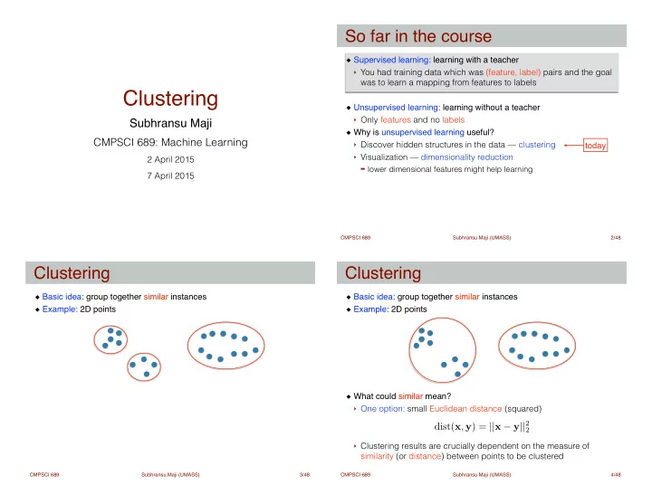
Basic idea: group together similar instances! Example: 2D points!

! ! ! ! ! !

What could similar mean?!

  • One option: small Euclidean distance (squared)

! !

  • Clustering results are crucially dependent on the measure of

similarity (or distance) between points to be clustered

Clustering

4

dist(x, y) = ||x − y||2

2

slide-2
SLIDE 2

Subhransu Maji (UMASS) CMPSCI 689 /48

Simple clustering: organize elements into k groups!

  • K-means
  • Mean shift
  • Spectral clustering

! ! !

Hierarchical clustering: organize elements into a hierarchy!

  • Bottom up - agglomerative
  • Top down - divisive

Clustering algorithms

5 Subhransu Maji (UMASS) CMPSCI 689 /48

Image segmentation: break up the image into similar regions

Clustering examples

6

image credit: Berkeley segmentation benchmark

Subhransu Maji (UMASS) CMPSCI 689 /48

Clustering news articles

Clustering examples

7 Subhransu Maji (UMASS) CMPSCI 689 /48

Clustering queries

Clustering examples

8

slide-3
SLIDE 3

Subhransu Maji (UMASS) CMPSCI 689 /48

Clustering people by space and time

Clustering examples

9

image credit: Pilho Kim

Subhransu Maji (UMASS) CMPSCI 689 /48

Clustering species (phylogeny)

Clustering examples

10

[K. Lindblad-Toh, Nature 2005]

phylogeny of canid species (dogs, wolves, foxes, jackals, etc)

Subhransu Maji (UMASS) CMPSCI 689 /48

Given (x1, x2, …, xn) partition the n observations into k (≤ n) sets S = {S1, S2, …, Sk} so as to minimize the within-cluster sum of squared distances

!

The objective is to minimize:

Clustering using k-means

11

arg min

S k

X

i=1

X

x∈Si

||x − µi||2 cluster center

Subhransu Maji (UMASS) CMPSCI 689 /48

Initialize k centers by picking k points randomly among all the points! Repeat till convergence (or max iterations)!

  • Assign each point to the nearest center (assignment step)

! ! !

  • Estimate the mean of each group (update step)

Lloyd’s algorithm for k-means

12

arg min

S k

X

i=1

X

x∈Si

||x − µi||2 arg min

S k

X

i=1

X

x∈Si

||x − µi||2

slide-4
SLIDE 4

Subhransu Maji (UMASS) CMPSCI 689 /48

k-means in action

13 http://simplystatistics.org/2014/02/18/k-means-clustering-in-a-gif/ Subhransu Maji (UMASS) CMPSCI 689 /48

k-means++ Guaranteed to converge in a finite number of iterations!

  • The objective decreases monotonically over time
  • Local minima if the partitions don’t change. Since there are finitely

many partitions, k-means algorithm must converge

!

Running time per iteration!

  • Assignment step: O(NKD)
  • Computing cluster mean: O(ND)

!

Issues with the algorithm:!

  • Worst case running time is super-polynomial in input size
  • No guarantees about global optimality

➡ Optimal clustering even for 2 clusters is NP-hard [Aloise et al., 09]

Properties of the Lloyd’s algorithm

14 Subhransu Maji (UMASS) CMPSCI 689 /48

A way to pick the good initial centers!

  • Intuition: spread out the k initial cluster centers

The algorithm proceeds normally once the centers are initialized! k-means++ algorithm for initialization:! 1.Chose one center uniformly at random among all the points 2.For each point x, compute D(x), the distance between x and the nearest center that has already been chosen 3.Chose one new data point at random as a new center, using a weighted probability distribution where a point x is chosen with a probability proportional to D(x)2 4.Repeat Steps 2 and 3 until k centers have been chosen

!

[Arthur and Vassilvitskii’07] The approximation quality is O(log k) in expectation

k-means++ algorithm

15

http://en.wikipedia.org/wiki/K-means%2B%2B

Subhransu Maji (UMASS) CMPSCI 689 /48

k-means for image segmentation

16

Grouping pixels based

  • n intensity similarity

feature space: intensity value (1D) K=2 K=3

slide-5
SLIDE 5

Subhransu Maji (UMASS) CMPSCI 689 /48

One issue with k-means is that it is sometimes hard to pick k! The mean shift algorithm seeks modes or local maxima of density in the feature space — automatically determines the number of clusters

Clustering using density estimation

17

K(x) = 1 Z X

i

exp ✓ −||x − xi||2 h ◆

Kernel density estimator Small h implies more modes (bumpy distribution)

Subhransu Maji (UMASS) CMPSCI 689 /48

Mean shift procedure:!

  • For each point, repeat till convergence
  • Compute mean shift vector
  • Translate the kernel window by m(x)#

Simply following the gradient of density

Mean shift algorithm

18

2 1 2 1

( )

n i i i n i i

g h g h

= =

! " # $ % & ' ( ' ( % & ) * = − % & # $ % & ' ( % & ' ( ) * ,

x - x x m x x x - x

exp ✓ −||x − xi||2 h ◆

Slide&by&Y.&Ukrainitz&&&B.&Sarel Subhransu Maji (UMASS) CMPSCI 689 /48

Search
 window Center of mass Mean Shift vector

Mean shift

19 Slide&by&Y.&Ukrainitz&&&B.&Sarel Subhransu Maji (UMASS) CMPSCI 689 /48

Search
 window Center of mass Mean Shift vector

Mean shift

20 Slide&by&Y.&Ukrainitz&&&B.&Sarel

slide-6
SLIDE 6

Subhransu Maji (UMASS) CMPSCI 689 /48

Search
 window Center of mass Mean Shift vector

Mean shift

21 Slide&by&Y.&Ukrainitz&&&B.&Sarel Subhransu Maji (UMASS) CMPSCI 689 /48

Search
 window Center of mass Mean Shift vector

Mean shift

22 Slide&by&Y.&Ukrainitz&&&B.&Sarel Subhransu Maji (UMASS) CMPSCI 689 /48

Search
 window Center of mass Mean Shift vector

Mean shift

23 Slide&by&Y.&Ukrainitz&&&B.&Sarel Subhransu Maji (UMASS) CMPSCI 689 /48

Search
 window Center of mass Mean Shift vector

Mean shift

24 Slide&by&Y.&Ukrainitz&&&B.&Sarel

slide-7
SLIDE 7

Subhransu Maji (UMASS) CMPSCI 689 /48

Search
 window Center of mass

Mean shift

25 Slide&by&Y.&Ukrainitz&&&B.&Sarel Subhransu Maji (UMASS) CMPSCI 689 /48

Cluster all data points in the attraction basin of a mode! Attraction basin is the region for which all trajectories lead to the same mode — correspond to clusters

Mean shift clustering

26 Slide&by&Y.&Ukrainitz&&&B.&Sarel Subhransu Maji (UMASS) CMPSCI 689 /48

Feature: L*u*v* color values! Initialize windows at individual feature points! Perform mean shift for each window until convergence! Merge windows that end up near the same “peak” or mode

Mean shift for image segmentation

27 Subhransu Maji (UMASS) CMPSCI 689 /48

Mean shift clustering results

28

http://www.caip.rutgers.edu/~comanici/MSPAMI/msPamiResults.html

slide-8
SLIDE 8

Subhransu Maji (UMASS) CMPSCI 689 /48

Pros:!

  • Does not assume shape on clusters
  • One parameter choice (window size)
  • Generic technique
  • Finds multiple modes

Cons:!

  • Selection of window size
  • Is rather expensive: O(DN2) per iteration
  • Does not work well for high-dimensional features

Mean shift discussion

29 Kristen Grauman Subhransu Maji (UMASS) CMPSCI 689 /48

Spectral clustering

30

[Shi & Malik ‘00; Ng, Jordan, Weiss NIPS ‘01]

Subhransu Maji (UMASS) CMPSCI 689 /48

Spectral clustering

31

[Figures from Ng, Jordan, Weiss NIPS ‘01]

Subhransu Maji (UMASS) CMPSCI 689 /48

Group points based on the links in a graph!

! ! ! !

How do we create the graph?!

  • Weights on the edges based on similarity between the points
  • A common choice is the Gaussian kernel

! !

One could create!

  • A fully connected graph
  • k-nearest graph (each node is connected only to its k-nearest

neighbors)

Spectral clustering

32

A B

slide credit: Alan Fern

W(i, j) = exp ✓ −||xi − xj||2 2σ2 ◆

slide-9
SLIDE 9

Subhransu Maji (UMASS) CMPSCI 689 /48

Consider a partition of the graph into two parts A and B!

! ! ! ! ! !

Cut(A, B) is the weight of all edges that connect the two groups!

! ! !

An intuitive goal is to find a partition that minimizes the cut!

  • min-cuts in graphs can be computed in polynomial time

Graph cut

33

Cut(A, B) = X

i∈A,j∈B

W(i, j) = 0.3

Subhransu Maji (UMASS) CMPSCI 689 /48

The weight of a cut is proportional to number of edges in the cut; tends to produce small, isolated components.

Problem with min-cut

34

[Shi & Malik, 2000 PAMI]

We would like a balanced cut

Subhransu Maji (UMASS) CMPSCI 689 /48

Let W(i, j) denote the matrix of the edge weights! The degree of node in the graph is:!

! ! ! ! ! !

The volume of a set A is defined as:

Graphs as matrices

35

d(i) = X

j

W(i, j) Vol(A) = X

i∈A

d(i)

Subhransu Maji (UMASS) CMPSCI 689 /48

Intuition: consider the connectivity between the groups relative to the volume of each group:!

! ! ! ! ! ! ! ! !

Unfortunately minimizing normalized cut is NP-Hard even for planar graphs [Shi & Malik, 00]

Normalized cut

36

NCut(A, B) = Cut(A, B) Vol(A) + Cut(A, B) Vol(B) NCut(A, B) = Cut(A, B) ✓Vol(A) + Vol(B) Vol(A)Vol(B) ◆

minimized when Vol(A) = Vol(B) ! encouraging a balanced cut

slide-10
SLIDE 10

Subhransu Maji (UMASS) CMPSCI 689 /48

We will formulate an optimization problem!

  • Let W be the similarity matrix
  • Let D be a diagonal matrix with D(i,i) = d(i) — the degree of node i
  • Let x be a vector {1, -1}N , x(i) = 1 i ∈ A
  • The matrix (D-W) is called the Laplacian of the graph

!

With some simplification we can show that the problem of minimizing normalized cuts can be written as:

Solving normalized cuts

37

min

x NCut(x) = min y

yT (D − W)y yT Dy subject to: yT D1 = 0 y(i) ∈ {1, −b}

Subhransu Maji (UMASS) CMPSCI 689 /48

Normalized cuts objective:!

! ! ! ! !

Relax the integer constraint on y:!

! !

Same as: (Generalized eigenvalue problem)! Note that , so the first eigenvector is y1 = 1, with the corresponding eigenvalue of 0! The eigenvector corresponding to the second smallest eigenvalue is the solution to the relaxed problem

Solving normalized cuts

38

min

x NCut(x) = min y

yT (D − W)y yT Dy subject to: yT D1 = 0 y(i) ∈ {1, −b} (D − W)y = λDy (D − W)1 = 0 min

y yT (D − W)y; subject to: yT Dy = 1, yT D1 = 0

Subhransu Maji (UMASS) CMPSCI 689 /48

Data: Gaussian weighted edges connected to 3 nearest neighbors

Spectral clustering example

39 Subhransu Maji (UMASS) CMPSCI 689 /48

Components of the eigenvector corresponding to the second smallest eigenvalue

Spectral clustering example

40

slide-11
SLIDE 11

Subhransu Maji (UMASS) CMPSCI 689 /48

The eigenvalue is real valued, so to obtain a split you may threshold it! How to pick the threshold?!

  • Pick the median value
  • Choose a threshold that minimizes the normalized cut objective

How to create multiple partitions?!

  • Recursively split each partition
  • Compute multiple eigenvalues and cluster them using k-means

➡ Example: multiple eigenvalues of an image and their gradients

Creating partitions from eigenvalues

41

http://ttic.uchicago.edu/~mmaire/papers/pdf/amfm_tpami2011.pdf

Subhransu Maji (UMASS) CMPSCI 689 /48

Hierarchical clustering

42 Subhransu Maji (UMASS) CMPSCI 689 /48

Organize elements into a hierarchy! Two kinds of methods:!

  • Agglomerative: a “bottom up” approach where elements start as

individual clusters and clusters are merged as one moves up the hierarchy

  • Divisive: a “top down” approach where elements start as a single

cluster and clusters are split as one moves down the hierarchy

Hierarchical clustering

43 Subhransu Maji (UMASS) CMPSCI 689 /48

Agglomerative clustering:!

  • First merge very similar instances
  • Incrementally build larger clusters out
  • f smaller clusters

Algorithm:!

  • Maintain a set of clusters
  • Initially, each instance in its own

cluster

  • Repeat:

➡ Pick the two “closest” clusters ➡ Merge them into a new cluster ➡ Stop when there’s only one cluster left

Produces not one clustering, but a family of clusterings represented by a dendrogram

Agglomerative clustering

44

slide-12
SLIDE 12

Subhransu Maji (UMASS) CMPSCI 689 /48

How should we define “closest” for clusters with multiple elements?!

!

Many options:!

  • Closest pair: single-link clustering
  • Farthest pair: complete-link clustering
  • Average of all pairs

Agglomerative clustering

45 Subhransu Maji (UMASS) CMPSCI 689 /48

Different choices create different clustering behaviors

Agglomerative clustering

46 Subhransu Maji (UMASS) CMPSCI 689 /48

Clustering is an example of unsupervised learning! Partitions or hierarchy! Several partitioning algorithms:!

  • k-means: simple, efficient and often works in practice

➡ k-means++ for better initialization

  • mean shift: modes of density

➡ slow but suited for problems with unknown number of clusters with

varying shapes and sizes

  • spectral clustering: clustering as graph partitions

➡ solve (D - W)x = λDx followed by k-means

Hierarchical clustering methods:!

  • Agglomerative or divisive

➡ single-link, complete-link and average-link

Summary

47 Subhransu Maji (UMASS) CMPSCI 689 /48

Slides adapted from David Sontag, Luke Zettlemoyer, Vibhav Gogate, Carlos Guestrin, Andrew Moore, Dan Klein, James Hays, Alan Fern, and Tommi Jaakkola!

!

Many images are from the Berkeley segmentation benchmark!

  • http://www.eecs.berkeley.edu/Research/Projects/CS/vision/bsds

!

Normalized cuts image segmentation:!

  • http://www.timotheecour.com/research.html

Slides credit

48