Clustering DSE 210 Clustering in R d Two common uses of clustering: - - PDF document

SLIDE 1

Clustering

DSE 210

Clustering in Rd

Two common uses of clustering:

• Vector quantization

Find a finite set of representatives that provides good coverage of a complex, possibly infinite, high-dimensional space.

• Finding meaningful structure in data

Finding salient grouping in data.

SLIDE 2

Widely-used clustering methods

1 K-means and its many variants 2 EM for mixtures of Gaussians 3 Agglomerative hierarchical clustering

The k-means optimization problem

• Input: Points x1, . . . , xn 2 Rd; integer k
• Output: “Centers”, or representatives, µ1, . . . , µk 2 Rd
• Goal: Minimize average squared distance between points and their

nearest representatives: cost(µ1, . . . , µk) =

n

X

i=1

min

j

kxi µjk2 The centers carve Rd up into k convex regions: µj’s region consists

• f points for which it is the closest

center.

SLIDE 3

Lloyd’s k-means algorithm

The k-means problem is NP-hard to solve. The most popular heuristic is called the “k-means algorithm”.

• Initialize centers µ1, . . . , µk in some manner.
• Repeat until convergence:
• Assign each point to its closest center.
• Update each µj to the mean of the points assigned to it.

Each iteration reduces the cost ) convergence to a local optimum.

Initializing the k-means algorithm

Typical practice: choose k data points at random as the initial centers. Another common trick: start with extra centers, then prune later. A particularly good initializer: k-means++

• Pick a data point x at random as the first center
• Let C = {x} (centers chosen so far)
• Repeat until desired number of centers is attained:
• Pick a data point x at random from the following distribution:

Pr(x) / dist(x, C)2, where dist(x, C) = minz∈C kx zk

• Add x to C

SLIDE 4

Representing images using k-means codewords

Given a collection of images, how to represent as fixed-length vectors?

patch of fixed size

• Look at all ` ⇥ ` patches in all images.
• Run k-means on this entire collection to get k centers.
• Now associate any image patch with its nearest center.
• Represent an image by a histogram over {1, 2, . . . , k}.

Such data sets are truly enormous.

Streaming and online computation

Streaming computation: for data sets that are too large to fit in memory.

• Make one pass (or maybe a few passes) through the data.
• On each pass:
• See data points one at a time, in order.
• Update models/parameters along the way.
• There is only enough space to store a tiny fraction of the data, or a

perhaps short summary. Online computation: an even more lightweight setup, for data that is continuously being collected.

• Initialize a model.
• Repeat forever:
• See a new data point.
• Update model if need be.

SLIDE 5

Example: sequential k-means

1 Set the centers µ1, . . . , µk to the first k data points 2 Set their counts to n1 = n2 = · · · = nk = 1 3 Repeat, possibly foreover:

• Get next data point x
• Let µj be the center closest to x
• Update µj and nj:

µj = njµj + x nj + 1 and nj = nj + 1

K-means: the good and the bad

The good:

• Fast and easy.
• Effective in quantization.

The bad:

• Geared towards data in which the clusters are spherical, and of

roughly the same radius. Is there is a similarly-simple algorithm in which clusters of more general shape are accommodated?

SLIDE 6

Mixtures of Gaussians

Idea: model each cluster by a Gaussian:

20% 20% 40% 20%

Each of the k clusters is specified by:

• a Gaussian distribution Pj = N(µj, Σj)
• a mixing weight ⇡j

Overall distribution over Rd: a mixture of Gaussians Pr(x) = ⇡1P1(x) + · · · + ⇡kPk(x)

The clustering task

Given data x1, . . . , xn 2 Rd, find the maximum-likelihood mixture of Gaussians: that is, find parameters

• ⇡1, . . . , ⇡k 0 summing to one
• µ1, . . . , µk 2 Rd
• Σ1, . . . , Σk 2 Rd⇥d

to maximize Pr (data | ⇡1P1 + · · · + ⇡kPk) =

n

Y

i=1

@

k

X

j=1

⇡jPj(xi) 1 A =

n

Y

i=1

@

k

X

j=1

⇡j (2⇡)p/2|Σj|1/2 exp ✓ 1 2(xi µj)TΣ1

j

(xi µj) ◆1 A where Pj is the distribution of the jth cluster, N(µj, Σj).

SLIDE 7

The EM algorithm

1 Initialize ⇡1, . . . , ⇡k and P1 = N(µ1, Σ1), . . . , Pk = N(µk, Σk) in

some manner.

2 Repeat until convergence:

• Assign each point xi fractionally between the k clusters:

wij = Pr(cluster j | xi) = πjPj(xi) P

` π`P`(xi)

• Now update the mixing weights, means, and covariances:

πj = 1 n

n

X

i=1

wij µj = 1 nπj

n

X

i=1

wijxi Σj = 1 nπj

n

X

i=1

wij(xi µj)(xi µj)T

Hierarchical clustering

Choosing the number of clusters (k) is difficult. Often there is no single right answer, because of multiscale structure. Hierarchical clustering avoids these problems.

SLIDE 8

Example: gene expression data The single linkage algorithm

• Start with each point in its own, singleton, cluster
• Repeat until there is just one cluster:
• Merge the two clusters with the closest pair of points
• Disregard singleton clusters

SLIDE 9

Linkage methods

• Start with each point in its own, singleton, cluster
• Repeat until there is just one cluster:
• Merge the two “closest” clusters

How to measure the distance between two clusters of points, C and C 0?

• Single linkage

dist(C, C 0) = min

x2C,x02C 0 kx x0k

• Complete linkage

dist(C, C 0) = max

x2C,x02C 0 kx x0k

Average linkage

Three commonly-used variants:

1 Average pairwise distance between points in the two clusters

dist(C, C 0) = 1 |C| · |C 0| X

x2C

X

x02C 0

kx x0k

2 Distance between cluster centers

dist(C, C 0) = kmean(C) mean(C 0)k

3 Ward’s method: the increase in k-means cost occasioned by merging

the two clusters dist(C, C 0) = |C| · |C 0| |C| + |C 0|kmean(C) mean(C 0)k2

SLIDE 10

DSE 210: Probability and statistics Winter 2018

Worksheet 9 — Clustering

• 1. For this problem, we’ll be using the animals with attributes data set. Go to

http://attributes.kyb.tuebingen.mpg.de and, under “Downloads”, choose the “base package” (the very first file in the list). Unzip it and look

• ver the various text files.
• 2. This is a small data set that has information about 50 animals. The animals are listed in classes.txt.

For each animal, the information consists of values for 85 features: does the animal have a tail, is it slow, does it have tusks, etc. The details of the features are in predicates.txt. The full data consists

• f a 50 × 85 matrix of real values, in predicate-matrix-continuous.txt. There is also a binarized

version of this data, in predicate-matrix-binary.txt.

• 3. Load the real-valued array, and also the animal names, into Python. Run k-means on the data (from

sklearn.cluster) and ask for k = 10 clusters. For each cluster, list the animals in it. Does the clustering make sense?

• 4. Now hierarchically cluster this data, using scipy.cluster.hierarchy.linkage.

Choose Ward’s method, and plot the resulting tree using the dendrogram method, setting the orientation parameter to ‘right’ and labeling each leaf with the corresponding animal name. You will run into a problem: the plot is too cramped because the default figure size is so small. To make it larger, preface your code with the following: from pylab import rcParams rcParams[’figure.figsize’] = 5, 10 (or try a different size if this doesn’t seem quite right). Does the hierarchical clustering seem sensible to you?

• 5. Turn in an iPython notebook with a transcript of all this experimentation.

9-1

SLIDE 11

Informative projections

DSE 210

Dimensionality reduction

Why reduce the number of features in a data set?

1 It reduces storage and computation time. 2 High-dimensional data often has a lot of redundancy. 3 Remove noisy or irrelevant features.

Example: are all the pixels in an image equally informative? If we were to choose a few pixels to discard, which would be the prime can- didates?

SLIDE 12

Eliminating low variance coordinates

MNIST: what fraction of the total variance lies in the 100 (or 200, or 300) coordinates with lowest variance?

The effect of correlation

Suppose we wanted just one feature for the following data. This is the direction of maximum variance.

SLIDE 13

Comparing projections Projection: formally

What is the projection of x 2 Rd in the direction u 2 Rd? Assume u is a unit vector (i.e. kuk = 1).

x · u u x

Projection is x · u = u · x = uTx =

d

X

i=1

uixi.

SLIDE 14

Examples

What is the projection of x = ✓2 3 ◆ along the following directions?

1 The x1-axis? 2 The direction of

✓ 1 1 ◆ ?

The best direction

Suppose we need to map our data x 2 Rd into just one dimension: x 7! u · x for some unit direction u 2 Rd What is the direction u of maximum variance? Useful fact 1:

• Let Σ be the d ⇥ d covariance matrix of X.
• The variance of X in direction u (the variance of X · u) is:

uTΣu.

SLIDE 15

Best direction: example

Here covariance matrix Σ = ✓ 1 0.85 0.85 1 ◆

The best direction

Suppose we need to map our data x 2 Rd into just one dimension: x 7! u · x for some unit direction u 2 Rd What is the direction u of maximum variance? Useful fact 1:

• Let Σ be the d ⇥ d covariance matrix of X.
• The variance of X in direction u is given by uTΣu.

Useful fact 2:

• uTΣu is maximized by setting u to the first eigenvector of Σ.
• The maximum value is the corresponding eigenvalue.

SLIDE 16

Best direction: example

Direction: first eigenvector of the 2 ⇥ 2 covariance matrix of the data. Projection onto this direction: the top principal component of the data

Projection onto multiple directions

Projecting x 2 Rd into the k-dimensional subspace defined by vectors u1, . . . , uk 2 Rd. This is easiest when the ui’s are orthonormal:

• They have length one.
• They are at right angles to each other: ui · uj = 0 when i 6= j

The projection is a k-dimensional vector: (x · u1, x · u2, . . . , x · uk) = B B B @

• u1
• !
• u2
• !

. . .

• uk
• !

1 C C C A | {z }

call this UT

B B @ x ? ? x ? ? y 1 C C A U is the d ⇥ k matrix with columns u1, . . . , uk.

SLIDE 17

Projection onto multiple directions: example

E.g. project data in R4 onto the first two coordinates. Take vectors u1 = B B @ 1 1 C C A , u2 = B B @ 1 1 C C A (notice: orthonormal) Write UT = ✓

• u1
• !
• u2
• !

◆ = ✓ 1 1 ◆ The projection of x 2 R4 is UTx = ✓x1 x2 ◆

The best k-dimensional projection

Let Σ be the d ⇥ d covariance matrix of X. In O(d3) time, we can compute its eigendecomposition, consisting of

• real eigenvalues λ1 λ2 · · · λd
• corresponding eigenvectors u1, . . . , ud 2 Rd that are orthonormal

(unit length and at right angles to each other) Fact: Suppose we want to map data X 2 Rd to just k dimensions, while capturing as much of the variance of X as possible. The best choice of projection is: x 7! (u1 · x, u2 · x, . . . , uk · x), where ui are the eigenvectors described above. This projection is called principal component analysis (PCA).

SLIDE 18

Example: MNIST

Contrast coordinate projections with PCA:

Applying PCA to MNIST: examples

Reconstruct this original image from its PCA projection to k dimensions. k = 200 k = 150 k = 100 k = 50 How do we get these reconstructions?

SLIDE 19

Reconstruction from a 1-d projection

Projection onto R: Reconstruction in R2:

Reconstruction from projection onto multiple directions

Projecting into the k-dimensional subspace defined by orthonormal u1, . . . , uk ∈ Rd. The projection of x is a k-dimensional vector: (x · u1, x · u2, . . . , x · uk) = B B B @ ← − − − − − u1 − − − − − → ← − − − − − u2 − − − − − → . . . ← − − − − − uk − − − − − → 1 C C C A | {z }

call this UT

B B @ x ? ? x ? ? y 1 C C A The reconstruction from this projection is: (x · u1)u1 + (x · u2)u2 + · · · + (x · uk)uk = UUTx.

SLIDE 20

MNIST: image reconstruction

Reconstruct this original image x from its PCA projection to k dimensions. k = 200 k = 150 k = 100 k = 50 Reconstruction UUTx, where U’s columns are top k eigenvectors of Σ.

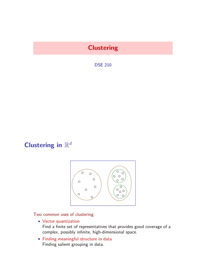
Case study: personality assessment

What are the dimensions along which personalities differ?

• Lexical hypothesis: most important personality characteristics have

become encoded in natural language.

• Allport and Odbert (1936): identified 4500 words describing

personality traits.

• Group these words into (approximate) synonyms, by manual

clustering. E.g. Norman (1967):

1218

LEWIS R. GOLDBERG Table 1

The 75 Categories in the Norman Taxonomy of 1,431 Trait-Descriptive Adjectives

No. Factor pole/category Examples terms

Reliability a

I+ Spirit Jolly, merry, witty, lively, peppy 26 Talkativeness Talkative, articulate, verbose, gossipy 23 Sociability Companionable, social, outgoing 9 Spontaneity Impulsive, carefree, playful, zany 28 Boisterousness Mischievous, rowdy, loud, prankish 11 Adventure Brave, venturous, fearless, reckless 44 Energy Active, assertive, dominant, energetic 36 Conceit Boastful, conceited, egotistical 13 Vanity Affected, vain, chic, dapper, jaunty 5 Indiscretion Nosey, snoopy, indiscreet, meddlesome 6 Sensuality Sexy, passionate, sensual, flirtatious 12 I- Lethargy Reserved, lethargic, vigorless, apathetic 19 Aloofness Cool, aloof, distant, unsocial, withdrawn 26 Silence Quiet, secretive, untalkative, indirect 22 Modesty Humble, modest, bashful, meek, shy 18 Pessimism Joyless, solemn, sober, morose, moody 19 Unfriendliness Tactless, thoughtless, unfriendly 20 II+ Trust Trustful, unsuspicious, unenvious 20 Amiability Democratic, friendly, genial, cheerful 29 Generosity Generous, charitable, indulgent, lenient 18 Agreeableness Conciliatory, cooperative, agreeable 17 Tolerance Tolerant, reasonable, impartial, unbiased 19 Courtesy Patient, moderate, tactful, polite, civil 17 Altruism Kind, loyal, unselfish, helpful, sensitive 29 Warmth Affectionate, warm, tender, sentimental 18 Honesty Moral, honest, just, principled 16 II- Vindictiveness Sadistic, vengeful, cruel, malicious 13 Ill humor Bitter, testy, crabby, sour, surly 16 Criticism Harsh, severe, strict, critical, bossy 33 Disdain Derogatory, caustic, sarcastic, catty 16 Antagonism Negative, contrary, argumentative I l Aggressiveness Belligerent, abrasive, unruly, aggressive 21 Dogmatism Biased, opinionated, stubborn, inflexible 49 Temper Irritable, explosive, wild, short-tempered 29 Distrust Jealous, mistrustful, suspicious 8 Greed Stingy, selfish, ungenerous, envious 18 Dishonesty Scheming, sly, wily, insincere, devious 29 III+ Industry Persistent, ambitious, organized, thorough 43 Order Orderly, prim, tidy 3 Self-discipline Discreet, controlled, serious, earnest 17 Evangelism Crusading, zealous, moralistic, prudish 13 Consistency Predictable, rigid, conventional, rational 27 Grace Courtly, dignified, genteel, suave 8 Reliability Conscientious, dependable, prompt, punctual 11 Sophistication Blas6, urbane, cultured, refined 16 Formality Formal, pompous, smug, proud 13 Foresight Aimful, calculating, farseeing, progressive 17 Religiosity Mystical, devout, pious, spiritual 13 Maturity Mature 1 Passionlessness Coy, demure, chaste, unvoluptuous 4 Thrift Economical, frugal, thrifty, unextravagant 4 III- Negligence Messy, forgetful, lazy, careless 51 Inconsistency Changeable, erratic, fickle, absent-minded 17 Rebelliousness Impolite, impudent, rude, cynical 22 Irreverence Nonreligious, informal, profane 9 Provinciality Awkward, unrefined, earthy, practical 27 Intemperance Thriftless, excessive, self-indulgent 13 .88 .86 .77 .77 .78 .86 .77 .76 .28 .55 .76 .74 .86 .87 .76 .79 .70 .83 .81 .70 .71 .76 .73 .76 .82 .67 .79 .75 .79 .74 .75 .79 .78 .86 .65 .61 .80 .85 .62 .64 .71 .77 .73 .68 .72 .67 .62 .86 .13 .74 .90 .72 .81 .73 .63 .67 .22 .21 .27 .11 .24 .12 .08 .20 .07 .17 .20 .13 .19 .23 .15 .17 .10 .19 .13 .11 .13 .14 .14 .10 .20 .11 .22 .16 .10 .15 .21 .15 .07 .17 .19 .08 .12 .12 .35 .10 .16 .11 .26 .16 .14 .13 .09 .31 .04 .42 .14 .13 .16 .23 .06 .13

• Data collection: subjects whether these words describe them.

SLIDE 21

Personality assessment: the data

Matrix of data (1 = strongly disagree, 5 = strongly agree) shy merry tense boastful forgiving quiet Person 1 4 1 1 2 5 5 Person 2 1 4 4 5 2 1 Person 3 2 4 5 4 2 2 . . . How to extract important directions?

• Treat each column as a data point, find tight clusters
• Treat each row as a data point, apply PCA
• Or factor analysis, independent component analysis, etc.

What would PCA accomplish?

E.g.: Suppose two traits (generosity, trust) are so highly correlated that each person either answers “1” to both or “5” to both.

1 5 1 5 generosity trust

A single PCA dimension would entirely account for both traits.

SLIDE 22

Personality assessment: the data

Matrix of data (1 = strongly disagree, 5 = strongly agree) shy merry tense boastful forgiving quiet Person 1 4 1 1 2 5 5 Person 2 1 4 4 5 2 1 Person 3 2 4 5 4 2 2 . . . Methodology: apply PCA to the rows of this matrix.

The “Big Five” taxonomy

Extraversion −: quiet (-.83), reserved (-.80), shy (-.75), silent (-.71) +: talkative (.85), assertive (.83), active (.82), energetic (.82) Agreeableness −: fault-finding (-.52), cold (-.48), unfriendly (-.45), quarrelsome (-.45) +: sympathetic (.87), kind (.85), appreciative (.85), affectionate (.84) Conscientousness −: careless (-.58), disorderly (-.53), frivolous (-.50), irresponsible (-.49) +: organized (.80), thorough (.80), efficient (.78), responsible (.73) Neuroticism −: stable (-.39), calm (-.35), contented (-.21) +: tense (.73), anxious (.72), nervous (.72), moody (.71) Openness −: commonplace (-.74), narrow (-.73), simple (-.67), shallow (-.55) +: imaginative (.76), intelligent (.72), original (.73), insightful (.68)

SLIDE 23

Singular value decomposition

DSE 210

Moving between coordinate systems

e1 e2 u1 u2

SLIDE 24

The linear function defined by a matrix

• Any matrix M defines a linear function, x 7! Mx.

If M is a d ⇥ d matrix, this maps Rd to Rd.

• This function is easy to understand when M is diagonal:

@ 2 1 10 1 A | {z }

M

@ x1 x2 x3 1 A | {z }

x

= @ 2x1 x2 10x3 1 A | {z }

Mx

In this case, M simply scales each coordinate separately.

• General symmetric matrices also just scale coordinates separately...

but in a different coordinate system!

Eigenvector and eigenvalue: definition

Let M be a d ⇥ d matrix. We say u 2 Rd is an eigenvector of M if Mu = λu for some scaling constant λ. This λ is the eigenvalue associated with u. Key point: M maps eigenvector u onto the same direction.

SLIDE 25

Question: What are the eigenvectors and eigenvalues of: M =   2 −1 10   ?

Eigenvectors of a real symmetric matrix

Fact: Let M be any real symmetric d × d matrix. Then M has

• d eigenvalues λ1, . . . , λd
• corresponding eigenvectors u1, . . . , ud ∈ Rd that are orthonormal

Can think of u1, . . . , ud as the axes of the natural coordinate system for M.

SLIDE 26

Example

M = ✓ 1 −2 −2 1 ◆ has eigenvectors u1 = 1 √ 2 ✓ 1 1 ◆ , u2 = 1 √ 2 ✓ −1 1 ◆

1 Are these orthonormal? 2 What are the corresponding eigenvalues?

Spectral decomposition

Fact: Let M be any real symmetric d × d matrix. Then M has

• rthonormal eigenvectors u1, . . . , ud ∈ Rd and corresponding eigenvalues

λ1, . . . , λd. Spectral decomposition: Another way to write M:

M = B B @ x ? ? x ? ? x ? ? u1 u2 · · · ud ? ? y ? ? y ? ? y 1 C C A | {z }

U: columns are eigenvectors

B B B @ λ1 · · · λ2 · · · . . . . . . ... . . . · · · λd 1 C C C A | {z }

Λ: eigenvalues on diagonal

B B B @ ← − − − − − u1 − − − − − → ← − − − − − u2 − − − − − → . . . ← − − − − − ud − − − − − → 1 C C C A | {z }

UT

Thus Mx = UΛUTx:

• UT rewrites x in the {ui} coordinate system
• Λ is a simple coordinate scaling in that basis
• U sends the scaled vector back into the usual coordinate basis

SLIDE 27

Apply to the matrix we saw earlier: M = ✓ 1 −2 −2 1 ◆

• Eigenvectors u1 =

1 √ 2 ✓1 1 ◆ , u2 = 1 √ 2 ✓−1 1 ◆

• Eigenvalues λ1 = −1, λ2 = 3.

M = ✓ 1 −2 −2 1 ◆ = 1 √ 2 ✓ 1 −1 1 1 ◆ | {z }

U

✓ −1 3 ◆ | {z }

Λ

1 √ 2 ✓ 1 1 −1 1 ◆ | {z }

UT

M ✓ 1 2 ◆ = UΛUT ✓ 1 2 ◆

1 2

e1 e2 u1 u2

SLIDE 28

Principal component analysis revisited

e1 e2 u1 u2

Data vectors X 2 Rd

• Covariance matrix Σ is d ⇥ d, symmetric.
• Eigenvalues λ1 λ2 · · · λd

Eigenvectors u1, . . . , ud.

• u1, . . . , ud: another basis for data.
• Variance of X in direction ui is λi.
• Projection to k dimensions:

x 7! (x · u1, . . . , x · uk). What is the covariance of the projected data?

Singular value decomposition (SVD)

For symmetric matrices, such as covariance matrices, we have seen:

• Results about existence of eigenvalues and eigenvectors
• The fact that the eigenvectors form an alternative basis
• The resulting spectral decomposition, which is used in PCA

But what about arbitrary matrices M 2 Rp×q? Any p ⇥ q matrix (say p  q) has a singular value decomposition: M = B @ x ? x ? u1 · · · up ? y ? y 1 C A | {z }

p × p matrix U

B @ σ1 · · · . . . ... . . . · · · σp 1 C A | {z }

p × p matrix Λ

B @

• v1
• !

. . .

• vp
• !

1 C A | {z }

p × q matrix V T

• u1, . . . , up are orthonormal vectors in Rp
• v1, . . . , vp are orthonormal vectors in Rq
• σ1 σ2 · · · σp are singular values

SLIDE 29

Matrix approximation

We can factor any p × q matrix as M = UW T: M = B @ x ? x ? u1 · · · up ? y ? y 1 C A B @ σ1 · · · . . . ... . . . · · · σp 1 C A B @ ← − − − − − v1 − − − − − → . . . ← − − − − − vp − − − − − → 1 C A = B @ x ? x ? u1 · · · up ? y ? y 1 C A | {z }

p × p matrix U

B @ ← − − − − − σ1v1 − − − − − → . . . ← − − − − − σpvp − − − − − → 1 C A | {z }

p × q matrix W T

A concise approximation to M: just take the first k columns of U and the first k rows of W T, for k < p: b M = B @ x ? x ? u1 · · · uk ? y ? y 1 C A | {z }

p×k

@ ← − − − − − σ1v1 − − − − − → . . . ← − − − − − σkvk − − − − − → 1 A | {z }

k×q

Example: topic modeling

Blei (2012):

. , , . , , . . . gene dna genetic life evolve

• rganism

brain neuron nerve data number computer . , ,

Topics Documents Topic proportions and assignments

0.04 0.02 0.01 0.04 0.02 0.01 0.02 0.01 0.01 0.02 0.02 0.01 data number computer . , , 0.02 0.02 0.01

SLIDE 30

Latent semantic indexing (LSI)

Given a large corpus of n documents:

• Fix a vocabulary, say of V words.
• Bag-of-words representation for documents: each document

becomes a vector of length V , with one coordinate per word.

• The corpus is an n × V matrix, one row per document.

cat dog house boat garden · · · Doc 1 4 1 1 2 Doc 2 3 1 Doc 3 1 3 . . . Let’s find a concise approximation to this matrix M.

Latent semantic indexing, cont’d

Use SVD to get an approximation to M: for small k, B B B B B @ ← − − doc 1 − − → ← − − doc 2 − − → ← − − doc 3 − − → . . . ← − − doc n − − → 1 C C C C C A | {z }

n × V matrix M

≈ B B B B B @ ← − − θ1 − − → ← − − θ2 − − → ← − − θ3 − − → . . . ← − − θn − − → 1 C C C C C A | {z }

n × k matrix Θ

@ ← − − − − − Ψ1 − − − − − → . . . ← − − − − − Ψk − − − − − → 1 A | {z }

k × V matrix Ψ

Think of this as a topic model with k topics.

• Ψj is a vector of length V describing topic j: coefficient Ψjw is large

if word w appears often in that topic.

• Each document is a combination of topics: θij is the weight of topic

j in document i. Document i originally represented by ith row of M, a vector in RV . Can instead use θi ∈ Rk, a more concise “semantic” representation.

SLIDE 31

The rank of a matrix

Suppose we want to approximate a matrix M by a simpler matrix b M. What is a suitable notion of “simple”?

• Let’s say M and b

M are p × q, where p ≤ q.

• Treat each row of b

M as a data point in Rq.

• We can think of the data as “simple” if it actually lies in a

low-dimensional subspace.

• If the rows lie in k-dimensional subspace, we say that b

M has rank k. The rank of a matrix is the number of linearly independent rows. Low-rank approximation: given M ∈ Rp×q and an integer k, find the matrix b M ∈ Rp×q that is the best rank-k approximation to M. That is, find b M so that

• b

M has rank ≤ k

• The approximation error P

i,j(Mij − b

Mij)2 is minimized. We can get b M directly from the singular value decomposition of M.

Low-rank approximation

Recall: Singular value decomposition of p × q matrix M (with p ≤ q): M = B @ x ? x ? u1 · · · up ? y ? y 1 C A B @ σ1 · · · . . . ... . . . · · · σp 1 C A B @ ← − − − − − v1 − − − − − → . . . ← − − − − − vp − − − − − → 1 C A

• u1, . . . , up is an orthonormal basis of Rp
• v1, . . . , vq is an orthonormal basis of Rq
• σ1 ≥ · · · ≥ σp are singular values

The best rank-k approximation to M, for any k ≤ p, is then b M = @ x ? x ? u1 · · · uk ? y ? y 1 A | {z }

p × k

@ σ1 · · · 0 . . . ... . . . 0 · · · σk 1 A | {z }

k × k

@ ← − − − − − v1 − − − − − → . . . ← − − − − − vk − − − − − → 1 A | {z }

k × q

SLIDE 32

Example: Collaborative filtering

Details and images from Koren, Bell, Volinksy (2009). Recommender systems: matching customers with products.

• Given: data on prior purchases/interests of users
• Recommend: further products of interest

Prototypical example: Netflix. A successful approach: collaborative filtering.

• Model dependencies between different products, and between

different users.

• Can give reasonable recommendations to a relatively new user.

Two strategies for collaborative filtering:

• Neighborhood methods
• Latent factor methods

Neighborhood methods

Joe #2 #3 #1 #4

SLIDE 33

Latent factor methods

R R R

• Geared

toward males Serious Escapist The Princess Diaries Braveheart Lethal Weapon Independence Day Ocean’s 11 Sense and Sensibility Gus Dave Geared toward females Amadeus The Lion King Dumb and Dumber The Color Purple

The matrix factorization approach

User ratings are assembled in a large matrix M: Star Wars Matrix Casablanca Camelot Godfather · · · User 1 5 5 2 User 2 3 4 5 User 3 5 . . .

• Not rated = 0, otherwise scores 1-5.
• For n users and p movies, this has size n × p.
• Most of the entries are unavailable, and we’d like to predict these.

Idea: Find the best low-rank approximation of M, and use it to fill in the missing entries.

SLIDE 34

User and movie factors

Best rank-k approximation is of the form M ≈ UW T: B B B B B @ ← − − user 1 − − → ← − − user 2 − − → ← − − user 3 − − → . . . ← − − user n − − → 1 C C C C C A | {z }

n × p matrix M

≈ B B B B B @ ← − − u1 − − → ← − − u2 − − → ← − − u3 − − → . . . ← − − un − − → 1 C C C C C A | {z }

n × k matrix U

@ x ? x ? x ? w1 w2 · · · wp ? y ? y ? y 1 A | {z }

k × p matrix W T

Thus user i’s rating of movie j is approximated as Mij ≈ ui · wj This “latent” representation embeds users and movies within the same k-dimensional space:

• Represent ith user by ui ∈ Rk
• Represent jth movie by wj ∈ Rk

Top two Netflix factors

• ฀
• ฀

–1.5 –1.0 –0.5 0.0 0.5 1.0 –1.5 –1.0 –0.5 0.0 0.5 1.0 1.5 Factor vector 1 Factor vector 2

F r e d d y G

• t

F i n g e r e d F r e d d y v s . J a s

• n

H a l f B a k e d R

• a

d T r i p T h e S

• u

n d

• f

M u s i c S

• p

h i e ’ s C h

• i

c e M

• n

s t r u c k M a i d i n M a n h a t t a n T h e W a y W e W e r e R u n a w a y B r i d e C

• y
• t

e U g l y T h e R

• y

a l T e n e n b a u m s P u n c h

• D

r u n k L

• v

e I H e a r t H u c k a b e e s A r m a g e d d

• n

C i t i z e n K a n e T h e W a l t

• n

s : S e a s

• n

1 S t e p m

• m

J u l i e n D

• n

k e y

• B
• y

S i s t e r A c t T h e F a s t a n d t h e F u r i

• u

s T h e W i z a r d

• f

O z K i l l B i l l : V

• l

. 1 S c a r f a c e N a t u r a l B

• r

n K i l l e r s A n n i e H a l l B e l l e d e J

• u

r L

• s

t i n T r a n s l a t i

• n

T h e L

• n

g e s t Y a r d B e i n g J

• h

n M a l k

• v

i c h C a t w

• m

a n

SLIDE 35

DSE 210: Probability and statistics Winter 2018

Worksheet 10 — PCA and SVD

• 1. Is the following set of vectors an orthonormal basis of R3? Explain why or why not.

@ 3 4 1 A , @ 4 3 1 A , @ 1 1 A

• 2. The following four figures show different 2-dimensional data sets. In each case, make a rough sketch
• f an ellipsoidal contour of the covariance matrix and indicate the directions of the first and second

eigenvectors (mark which is which).

• 3. Let u1, u2 2 Rd be two vectors with ku1k = ku2k = 1 and u1 · u2 = 0. Define

U = @ x ? x ? u1 u2 ? y ? y 1 A 10-1

SLIDE 36

DSE 210 Worksheet 10 — PCA and SVD Winter 2018 (a) What are the dimensions of each of the following?

• U
• U T
• UU T
• u1uT

1

(b) What are the differences, if any, between the following four mappings?

• x 7! (u1 · x, u2 · x)
• x 7! (u1 · x)u1 + (u2 · x)u2
• x 7! U T x
• x 7! UU T x
• 4. Recall the animals with attributes data set from Worksheet 9, which has information about 50 animals,

each represented as a vector in R85. We would like to visualize these animals in 2-d. Show how to do this with a PCA projection from R85 to R2. Show the position of each animal, and label them with their names. (Remember from Worksheet 9 how to enlarge the figure. This time you might want to ask for size 10,10.) Does this embedding seem sensible to you?

• 5. In lecture, we looked at the effect of projecting the MNIST data set of handwritten digits to lower-

dimension: from 784 to 200, 150, 100, 50 dimensions. We found that the reconstruction error was fairly low for 150-dimensional projections, but noticeable for 50-dimensional projections. We now investigate these issues further. (a) Let X 2 Rd have covariance matrix Σ. Suppose the eigenvalues of Σ are λ1 λ2 · · · λd, and suppose the corresponding eigenvectors are u1, u2, . . . , ud. Then it can be shown that X has an

• verall variance of λ1 + · · · + λd, and that when X is projected onto the top k eigenvectors, the

residual variance (the information that gets lost) is λk+1 +· · ·+λd. Therefore, for this projection, the fraction of lost information, intuitively speaking, is F(k) = λk+1 + · · · + λd λ1 + · · · + λd Compute these fractions for the MNIST data set, for k = 200, 150, 100, 50, 25. (b) Suppose we are allowed a different projection for each digit. We would then expect that we can project to an even lower dimension while maintaining roughly the same amount of information. Test whether this is true as follows: for each digit j = 0, 1, 2, . . . , 9,

• Obtain the PCA projection to k dimensions, for k = 200, 150, 100, 50, 25.
• Compute the fraction Fj(k), for each such value of k.
• Pick a random instance of the digit. Show the original digit as well as its reconstruction

at each of these five values of k. (Note: the original images have pixel values in the range 0-255, but this might not be true of the reconstructions; therefore, you may need to clip the reconstructed pixels to lie within this range before displaying the image.) Show all the fractions Fj(k) in a table. Which digit seems to be the most amenable to low- dimensional projection? 10-2