Clustering Aggregation Aristides Gionis, Heikki Mannila, and - - PDF document

Clustering Aggregation

Aristides Gionis, Heikki Mannila, and Panayiotis Tsaparas Helsinki Institute for Information Technology, BRU Department of Computer Science University of Helsinki, Finland first.lastname@cs.helsinki.fi Abstract

We consider the following problem: given a set of clus- terings, find a clustering that agrees as much as possible with the given clusterings. This problem, clustering aggre- gation, appears naturally in various contexts. For example, clustering categorical data is an instance of the problem: each categorical variable can be viewed as a clustering of the input rows. Moreover, clustering aggregation can be used as a meta-clustering method to improve the robustness

• f clusterings. The problem formulation does not require a-

priori information about the number of clusters, and it gives a natural way for handling missing values. We give a formal statement of the clustering-aggregationproblem, we discuss related work, and we suggest a number of algorithms. For several of the methods we provide theoretical guarantees on the quality of the solutions. We also show how sampling can be used to scale the algorithms for large data sets. We give an extensive empirical evaluation demonstrating the useful- ness of the problem and of the solutions.

1 Introduction

Clustering is an important step in the process of data analysis with applications to numerous fields. Informally, clustering is defined as the problem of partitioning data ob- jects into groups (clusters), such that objects in the same group are similar, while objects in different groups are dis- similar. This definition assumes that there is some well defined quality measure that captures intra-cluster similar- ity and/or inter-cluster dissimilarity, and then clustering be- comes the problem of grouping together data objects so that the quality measure is optimized. In this paper we propose a novel approach to clustering that is based on the concept of aggregation. We assume that given the data set we can obtain some information on how these points should be clustered. This information comes in the form of m clusterings C1, . . . , Cm. The objective is to

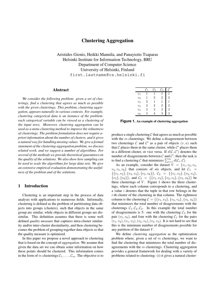
C1 C2 C3 C v1 1 1 1 1 v2 1 2 2 2 v3 2 1 1 1 v4 2 2 2 2 v5 3 3 3 3 v6 3 4 3 3

Figure 1. An example of clustering aggregation produce a single clustering C that agrees as much as possible with the m clusterings. We define a disagreement between two clusterings C and C′ as a pair of objects (v, u) such that C places them in the same cluster, while C′ places them in a different cluster, or vice versa. If d(C, C′) denotes the number of disagreements between C and C′, then the task is to find a clustering C that minimizes m

i=1 d(Ci, C).

As an example, consider the dataset V = {v1, v2, v3, v4, v5, v6} that consists of six objects, and let C1 = {{v1, v2}, {v3, v4}, {v5, v6}}, C2 = {{v1, v3}, {v2, v4}, {v5}, {v6}}, and C3 = {{v1, v3}, {v2, v4}, {v5, v6}} be three clusterings of V . Figure 1 shows the three cluster- ings, where each column corresponds to a clustering, and a value i denotes that the tuple in that row belongs in the i-th cluster of the clustering in that column. The rightmost column is the clustering C = {{v1, v3}, {v2, v4}, {v5, v6}} that minimizes the total number of disagreements with the clusterings C1, C2, C3. In this example the total number

• f disagreements is 5: one with the clustering C2 for the

pair (v5, v6), and four with the clustering C1 for the pairs (v1, v2), (v1, v3), (v2, v4), (v3, v4). It is not hard to see that this is the minimum number of disagreements possible for any partition of the dataset V . We define clustering aggregation as the optimization problem where, given a set of m clusterings, we want to find the clustering that minimizes the total number of dis- agreements with the m clusterings. Clustering aggregation provides a general framework for dealing with a variety of problems related to clustering: (i) it gives a natural cluster-

v4 v6 v5 v2 v1 v3 Figure 2.

Correlation clustering instance for the dataset in Figure 1. Solid edges indicate distances of 1/3, dashed edges indicate distances of 2/3, and dotted edges indicate distances of 1.

ing algorithm for categorical data, which allows for a simple treatment of missing values, (ii) it handles heterogeneous data, where tuples are defined over incomparable attributes, (iii) it determines the appropriate number of clusters and it detects outliers, (iv) it provides a method for improving the clustering robustness, by combining the results of many clustering algorithms, (v) it allows for clustering of data that is vertically partitioned in order to preserve privacy. We elaborate on the properties and the applications of cluster- ing aggregation in Section 2. The algorithms we propose for the problem of clustering aggregation take advantage of a related formulation, which is known as correlation clustering [2]. We map clustering aggregation to correlation clustering by considering the tu- ples of the dataset as vertices of a graph, and summariz- ing the information provided by the m input clusterings by weights on the edges of the graph. The weight of the edge (u, v) is the fraction of clusterings that place u and v in different clusters. For example, the correlation clus- tering instance for the dataset in Figure 1 is shown in Fig- ure 2. Note that if the weight of the edge (u, v) is less than 1/2 then the majority of the clusterings place u and v to- gether, while if the weight is greater than 1/2, the major- ity places u and v in different clusters. Ideally, we would like to cut all edges with weight more than 1/2, and not cut all edges with weight less than 1/2. The goal in corre- lation clustering is to find a partition of the vertices of the graph that it cuts as few as possible of the edges with low weight (less than 1/2), and as many as possible of the edges with high weight (more than 1/2). In Figure 2, clustering C = {{v1, v3}, {v2, v4}, {v5, v6}} is the optimal clustering. Clustering aggregation has has been previously consid- ered under a variety of names (consensus clustering, clus- tering ensemble, clustering combination) in a variety of dif- ferent areas: machine learning [19, 12], pattern recogni- tion [14], bio-informatics [13], and data mining [21, 5]. The problem of correlation clustering is interesting in its own right, and it has recently attracted a lot of attention in the theoretical computer-science community [2, 6, 8, 10]. We review some of the related literature on both clustering ag- gregation, and correlation clustering in Section 6. Our contributions can be summarized as follows.

• We formally define the problem of clustering aggrega-

tion, and we demonstrate the connection between clus- tering aggregation and correlation clustering.

• We present a number of algorithms for clustering ag-

gregation and correlation clustering. We also propose a sampling mechanism that allows our algorithms to handle large datasets. The problems we consider are NP-hard, yet we are still able to provide approxima- tion guarantees for many of the algorithms we propose. For the formulation of correlation clustering we con- sider we give a combinatorial 3-approximation algo- rithm, which is an improvement over the best known 9-approximation algorithm.

• We present an extensive experimental study, where we

demonstrate the benefits of our approach. Further- more, we show that our sampling technique reduces the running time of the algorithms, without sacrificing the quality of the clustering. The rest of this paper is structured as follows. In Sec- tion 2 we discuss the various applications of the clustering- aggregation framework, which is formally defined in Sec- tion 3. In Section 4 we describe in detail the proposed algorithms for clustering aggregation and correlation clus- tering, and the sampling-based algorithm that allows us to handle large datasets. Our experiments on synthetic and real datasets are presented in Section 5. Finally, Section 6 con- tains a review of the related work, and Section 7 is a short conclusion.

2 Applications of clustering aggregation

Clustering aggregationcan be applied in various settings. We will now present some of the main applications and fea- tures of our framework. Clustering categorical data: An important application

• f clustering aggregation is that it provides a very natural

method for clustering categorical data. Consider a dataset with tuples t1, . . . , tn over a set of categorical attributes A1, . . . , Am. The idea is to view each attribute Aj as a way of producing a simple clustering of the data: if Aj con- tains kj distinct values, then Aj partitions the data in kj clusters – one cluster for each value. Then, clustering ag- gregation considers all those m clusterings produced by the m attributes and tries to find a clustering that agrees as much as possible with all of them. 2

For example, consider a Movie database. Each tuple in the database corresponds to a movie that is defined over a set of attributes such as Director, Actor, Actress, Genre, Year, etc, some of which take categorical val-

• ues. Note that each of the categorical attributes defines nat-

urally a clustering. For example, the Movie.Genre at- tribute groups the movies according to their genre, while the Movie.Director according to who has directed the

• movie. The objective is to combine all these clusterings into

a single clustering. Clustering heterogeneous data: The clustering aggrega- tion method can be particularly effective in cases where the data are defined over heterogeneous attributes that contain incomparable values. Consider for example the case that there are many numerical attributes whose units are incom- parable (say, Movie.Budget and Movie.Year) and so it does not make sense to compare numerical vectors di- rectly using an Lp-type distance measure. A similar situa- tion arises in the case where the data contains a mix of cate- gorical and numerical values. In such cases the data can be partitioned vertically into sets of homogeneous attributes,

• btain a clustering for each of these sets by applying the

appropriate clustering algorithm, and then aggregate the in- dividual clusterings into a single clustering. Missing values: One of the major problems in clustering, and data analysis in general, is the issue of missing values. These are entries that for some reason (mistakes, omissions, lack of information) are incomplete. The clustering aggre- gation framework provides several ways for dealing with missing values in categorical data. One approach is to av- erage them out: an attribute that contains a missing value in some tuple does not have any information about how this tuple should be clustered, so we should let the remaining attributes decide. When computing the fraction of cluster- ings that disagree over a pair of tuples, we only consider the attributes that actually have a value on these tuples. Another approach, which we adopt in this paper, is to assume that given a pair of tuples for which an attribute contains at least one missing value, the attribute tosses a random coin and with probability p it reports the tuples as being clustered together, while with probability 1 − p it re- ports them as being in separate clusters. Each pair of tuples is treated independently. We are then interested in mini- mizing the expected number of disagreements between the clusterings. Identifying the correct number of clusters: One of the most important features of the formulation of clustering ag- gregation is that there is no need to specify the number of clusters in the result. The automatic identification of the appropriate number of clusters is a deep research problem that has attracted lots of attention [16, 18]. For most clus- tering approaches the quality (likelihood, sum of distances to cluster centers, etc.) of the solution improves as the num- ber of clusters is increased. Thus, the trivial solution of all singleton clusters is the optimal. There are two ways of handling the problem. The first is to have a hard constraint

• n the number of clusters, or on their quality. For example,

in agglomerative algorithms one can either fix in advance the number of clusters in the final clustering, or impose a bound on the distance beyond which no pair of clusters will be merged. The second approach is to use model selec- tion methods, e.g., Bayesian information criterion (BIC) or cross-validated likelihood [18] to compare models with dif- ferent numbers of clusters. The formulation of clustering aggregation takes automat- ically care of the selection of the number of clusters. If many input clusterings place two objects in the same clus- ter, then it will not be beneficial for a clustering-aggregation solution to split these two objects. Thus, the solution of all singleton clusters is not a trivial solution for our objective

• function. Furthermore, if there are k subsets of data objects

in the dataset, such that the majority of the input clusterings places them together, and separates them from the rest, then the clustering aggregation algorithm will correctly identify the k clusters, without any prior knowledge of k. Note that in the example in Figures 1 and 2 the optimal solution C discovers naturally a set of 3 clusters in the dataset. Indeed, the structure of the objective function ensures that the clustering aggregation algorithms will make their

• wn decisions, and settle naturally to the appropriate num-

ber of clusters. As we will show in our experimental sec- tion, our algorithms take advantage of this feature and for all

• ur datasets they generate clusterings with very reasonable

number of clusters. On the other hand, if the user insists on a predefined number of clusters, most of our algorithms can be easily modified to return that specific number of clus-

• ters. For example, the agglomerative algorithm described

in Section 4 can be made to continue merging clusters until the predefined number is reached. Detecting outliers: The ability to detect outliers is closely related with the ability to identify the correct number of

• clusters. If a node is not close to any other nodes, then, from

the point of view of the objective function, it would be bene- ficial to assign that node in a singleton cluster. In the case of categorical data clustering, the scenarios for detecting out- liers are very intuitive: if a tuple contains many uncommon values, it is does not participate in clusters with other tu- ples, and it will be identified as an outlier. Another scenario where it pays off to consider a tuple as an outlier is when the tuple contains common values (and therefore it participates in big clusters in the individual input clusterings) but there is no consensus to a common cluster (for example, a horror movie featuring actress Julia.Roberts and directed by the “independent” director Lars.vonTrier). 3

Improving clustering robustness: Different clustering al- gorithms have different qualities and different shortcom- ings. Some algorithms might perform well in specific datasets but not in others, or they might be very sensitive to parameter settings. For example, the single-linkage al- gorithm is good in identifying elongated regions but it is sensitive to clusters being connected with narrow strips of

• points. The k-means method is a widely-used algorithm,

but it is sensitive to clusters of uneven size, and it can get stuck in local optima. We suggest that by aggregating the results of different clustering we can improve significantly the robustness and the quality of the final clustering. The idea is that different algorithms make different “mistakes” that can be “canceled

• ut” in the final aggregation. Furthermore, for objects that

are outliers or noise, it is most likely that there will be no consensus on how they should be clustered, and thus they will be singled out by the aggregation algorithm. The intu- ition is similar to performing rank aggregation for improv- ing the results of web searches [9]. Our experiments in- dicate that clustering aggregation can improve significantly the results of individual algorithms. Privacy-preserving clustering: Consider a situation where a database table is vertically split and different attributes are maintained in different sites. Such a situation might arise in cases where different companies or governmental adminis- trations maintain various sets of data about a common pop- ulation of individuals. For such cases, our method offers a natural model for clustering the data maintained in all sites as a whole in a privacy-preserving manner, that is, without the need for the different sites to reveal their data to each

• ther, and without the need to rely on a trusted authority.

Each site clusters its own data independently and then all resulting clusterings are aggregated. The only information revealed is which tuples are clustered together; no informa- tion is revealed about data values of any individual tuples.

3 Description of the framework

We begin our discussion of the clustering aggregation framework by introducing our notation. Consider a set of n

• bjects V = {v1, . . . , vn}. A clustering C of V is a parti-

tion of V into k disjoint sets C1, . . . , Ck, that is, k

i Ci = V

and Ci ∩ Cj = ∅, for all i = j. The k sets C1, . . . , Ck are the clusters of C. For each v ∈ V we use C(v) to denote the label of the cluster to which the object v belongs. It is C(v) = j if and only if v ∈ Cj. In the sequel we consider m clusterings: we write Ci to denote i-th clustering, and ki for the number of clusters of Ci. In the clustering aggregation problem the task is to find a clustering that agrees as much as possible with a number

• f already-existing clusterings. To make the notion more

precise, we need to define a measure of disagreement be- tween clusterings. Consider first two objects u and v in V . The following simple 0/1 distance function checks if two clusterings C1 and C2 place u and v in the same clusters. du,v(C1, C2) =    1 if C1(u) = C1(v) and C2(u) = C2(v),

• r C1(u) = C1(v) and C2(u) = C2(v),
• therwise.

The distance between two clusterings C1 and C2 is defined as the number of pairs of objects on which the two cluster- ings disagree, that is, dV (C1, C2) =

• (u,v)∈V ×V

du,v(C1, C2). For the distance measure dV (·, ·) one can easily prove is that it satisfies the triangle inequality on the space of clusterings. We omit the proof due to space constraints. Observation 1 Given a set of objects V and clusterings C1, C2, C3 on V , we have dV (C1, C3) ≤ dV (C1, C2) + dV (C2, C3) The clustering aggregation problem can now be formalized as follows. Problem 1 (Clustering aggregation) Given a set of ob- jects V and m clusterings C1, . . . , Cm on V , compute a new clustering C that minimizes the total number of disagree- ments with all the given clusterings, i.e., it minimizes D(C) =

m

• i=1

dV (Ci, C). The clustering aggregation problem is also defined in [13], where it is shown to be NP-complete using the results of Barthelemy and Leclerc [3]. The algorithms we propose for the problem of clustering aggregation take advantage of a related formulation, which is known as correlation clustering [2]. Formally, correlation clustering is defined as follows. Problem 2 (Correlation clustering) Given a set of objects V , and distances Xuv ∈ [0, 1] for all pairs u, v ∈ V , find a partition C for the objects in V that minimizes the score function d(C) =

• (u,v)

C(u)=C(v)

Xuv +

• (u,v)

C(u)=C(v)

(1 − Xuv). 4

Correlation clustering is a generalization of clustering

• aggregation. Given the m clusterings C1, . . . , Cm as input
• ne can construct an instance of the correlation clustering

problem by defining the distances Xuv appropriately. In particular, let Xuv =

1 m · |{i | 1 ≤ i ≤ m and Ci(u) =

Ci(v)}| be the fraction of clusterings that assign the pair (u, v) into different clusters. For a candidate solution C of correlation clustering, if C places u, v in the same cluster it will disagree with mXuv of the original clusterings, while if C places u, v in different clusters it will disagree with the remaining m(1 − Xuv) clusterings. Thus, clustering aggre- gation can be reduced to correlation clustering, and as a re- sult correlation clustering is also an NP-complete problem. We note that an instance of correlation clustering produced by an instance of clustering aggregation is a restricted ver- sion of the correlation clustering problem. It is not hard to show that the values Xuv obey the triangle inequality, that is, Xuw ≤ Xuv + Xvw for all u, v and w in V . Since both problems we consider are NP-complete it is natural to seek algorithms with provable approximation

• guarantees. For the clustering aggregation problem, it is

trivial to obtain a 2-approximation solution. The idea is to take advantage of the triangle inequality property of the dis- tance measure dV (·, ·). Assume that we are given m objects in a metric space and we want to find a new point that min- imizes the sum of distances from the given objects. Then it is a well known fact that selecting the best among the m

• riginal objects yields a factor 2(1 − 1/m) approximate so-
• lution. For our problem, this method suggests taking as the

solution to clustering aggregation the clustering Ci that min- imizes D(Ci). Despite the small approximation factor, this solution is non-intuitive, and we observed that it does not work well in practice. The above algorithm cannot be used for the problem

• f correlation clustering – there are no input clusterings to

choose from. In general, the correlation clustering problem we consider is not equivalent to the clustering aggregation. There is an extensive literature in the theoretical computer science community on many different variants of the corre- lation clustering problem. We review some of these results in Section 6. Our problem corresponds to the weighted cor- relation clustering problem with linear cost functions [2], where the weights on the edges obey the triangle inequal-

• ity. The best known approximation algorithm for this case

can be obtained by combining the results of Bansal et al. [2] and Charikar et al. [6], giving an approximation ratio of 9. The algorithm does not take into account the fact that the weights obey the triangle inequality.

4 Algorithms

In this section we present the suggested algorithms for clustering aggregation. Most of our algorithms approach the problem through the correlation-clusteringproblem, and most of the algorithms are parameter-free. The BESTCLUSTERING algorithm: This is the trivial al- gorithm that was already mentioned in the previous sec-

• tion. Given m clusterings C1, . . . , Cm, BESTCLUSTERING

finds the clustering Ci from them that minimizes the total number of disagreements D(Ci). Using the data structures described in [3] the best clustering can be found in time O(mn). As discussed, this algorithm yields a solution with approximation ratio of at most 2(1 − 1/m). We can show that this bound is tight, that is, there exists an instance of the clustering aggregation problem, where the algorithm BEST- CLUSTERING produces a solution that is exactly 2(1−1/m) worse than the optimal. The proof of the lower bound ap- pears in the full version of the paper. The algorithm is specific to clustering aggregation—it cannot be used for correlation clustering. An interesting approach to the correlation clustering problem that might lead to a better approximation algorithm is to reconstruct m clusterings from the input distance matrix [Xuv]. Unfortu- nately, we are not aware of a polynomial-time algorithm for this problem of decomposition into clusterings. The BALLS algorithm: The BALLS algorithm works on the correlation clustering problem, and thus, it takes as input the matrix of pairwise distances Xuv. Equivalently, we view the input as a graph whose vertices are the tuples of a dataset, and the edges are weighted by the distances Xuv. The algorithm is defined with an input parameter α, and it is the only algorithm that requires an input parameter. By the theoretical analysis we sketch below, we can set the pa- rameter α to a constant value. However, different values of α can lead to better solutions in practice. The intuition of the algorithm is to find a set of ver- tices that are close to each other and far from other vertices. Given such a set, we consider it to be a cluster, we remove it from the graph, and we proceed with the rest of the vertices. The difficulty lies in finding such a set, since in principle any subset of the vertices can be a candidate. We overcome the difficulty by resorting again to the triangle inequality— this time for the distances Xuv. In order to find a good cluster we take all vertices that are close (within a “ball”) to a vertex u. The triangle inequality guarantees that if two vertices are close to u, then they are also relatively close to each other. We also note that it is intuitive that good clusters should be ball-shaped: since our cost function penalizes for long edges that are not cut, we do not expect to have elon- gated clusters in the optimal solution. More formally the algorithm is described as follows. It first sorts the vertices in increasing order of the total weight

• f the edges incident on each vertex, a heuristic that we ob-

served to work well in practice. At every step, the algo- rithm picks the first unclustered node u in that ordering. It 5

then finds the set of nodes S that are at a distance of at most 1/2 from the node u, and it computes the average dis- tance d(u, S) of the nodes in S to node u. If d(u, S) ≤ α then the nodes in S ∪ {u} are considered to form a cluster,

• therwise, node u forms a singleton cluster.

The cost of BALLS algorithm is guaranteed to be at most 3 times the cost of the optimal clustering. This result im- proves the previously best-known 9 approximation. The proof is defered to the full version of the paper, and here we give only a short sketch. Theorem 1 For α =

1 4, the approximation ratio of the

BALLS algorithm is at most 3. Sketch of the proof: The proof proceeds by bounding the cost that the algorithm pays for each edge (u, v) in terms of the cost that the optimal algorithm pays for the same edge. We make use of the fact that for an edge of distance c, if the algorithm takes the edge, then it pays at most c/(1 − c) times the cost of the optimal, while if it does not take the edge then it pays at most (1−c)/c times the optimal cost. It follows that taking an edge of cost less than 1/2, or splitting an edge of cost more than 1/2 is an optimal decision. Given a node u, if the BALLS algorithm decides to place u into a singleton cluster, then this means that

i∈S Xui ≥ 1 4|S|. Therefore, the cost paid by BALLS is at most 3 4|S|.

At the same time, since the weight of all edges (u, i), for i ∈ S is less than 1/2, the optimal algorithm takes all edges and pays at least 1

4|S|, giving approximation ratio 3.

In the case that the algorithm creates the cluster C = S ∪ {u} the decision to merge edges (u, i) for i ∈ S, and split the edges (u, j) for j ∈ S is optimal. We need to con- sider the edges Xij where i, j ∈ S, or i ∈ S and j ∈ S. We consider the case that i, j ∈ S; the other case is handled

• symmetrically. We sort the nodes in order of increasing dis-

tance from node u, and for each node j we consider the cost

• f all edges Xij with i < j. First, we note that if Xuj ≤ 1

4

then Xij ≤ Xui + Xuj ≤ 1

2, so the decision of the algo-

rithm to take edge (i, j) is optimal. For Xuj > 1

4, let Cj

denote the set of nodes i, where i < j. A key observation is that

i∈Cj Xui ≤ 1 4|Cj|: since we omit only edges with

high cost, the average cost cannot be more than 1

• 4. Using the

triangle inequality we can prove that

i∈Cj Xij ≤ 3 4|Cj|,

that is, the sum of Xij for i ∈ Cj is also small. This im- plies that the optimal algorithm cannot gain a lot by split- ting some of the Xij edges. The cost of the optimal can be shown to be at least 1

4|Cj|, giving again approximation

ratio 3.

• There are special cases where it is possible to prove a bet-

ter approximation ratio. For the case that m = 3 it is easy to show that the cost of the BALLS algorithm is at most 2 times that of the optimal solution. The complexity of the al- gorithm is O(mn2) for generating the table and O(n2) for running the algorithm. In our experiments we have observed that the value 1

4

tends to be small as it creates many singleton clusters. For many of our real datasets we have found that α = 2

5 leads

to better solutions. The AGGLOMERATIVE algorithm: The AGGLOMERA-

TIVE algorithm is a standard bottom-up algorithm for the

correlation clustering problem. It starts by placing every node into a singleton cluster. It then proceeds by consider- ing the pair of clusters with the smallest average distance. The average distance between two clusters is defined as the average weight of the edges between the two clusters. If the average distance of the closest pair of clusters is less than 1/2 then the two clusters are merged into a single cluster. If there are no two clusters with average distance smaller than 1/2, then no merging of current clusters can lead to a so- lution with improved cost d(C). Thus, the algorithm stops, and it outputs the clusters it has created so far. The AGGLOMERATIVE algorithm has the desirable fea- ture that it creates clusters where the average distance of any pair of nodes is at most 1/2. The intuition is that the

• pinion of the majority is respected on average. Using this

property we are able to prove that when m = 3, the AG-

GLOMERATIVE algorithm produces a solution with cost at

most 2 times that of the optimal solution. The complex- ity of the algorithm is O(mn2) for creating the matrix plus O(n2 log n) for running the algorithm. The FURTHEST algorithm: The FURTHEST algorithm is a top-down algorithm that works on the clustering correlation

• problem. It is inspired by the furthest-first traversal algo-

rithm, for which Hochbaum and Shmoys [17] showed that it achieves a 2-approximation for the clustering formulation

• f p-centers. As the BALLS algorithm uses a notion of a

“center” to find clusters and repeatedly remove them from the graph, the FURTHEST algorithm uses “centers” to parti- tion the graph in a top-down fashion. The algorithm starts by placing all nodes into a single

• cluster. Then it finds the pair of nodes that are furthest apart,

and places them into different clusters. These two nodes become the centers of the clusters. The remaining nodes are assigned to the center that incurs the least cost. This procedure is repeated iteratively: at each step a new center is generated that is the furthest from the existing centers, and the nodes are assigned to the center that incurs the least

• cost. At the end of each step, the cost of the new solution is
• computed. If it is lower than that of the previous step then

the algorithm continues. Otherwise, the algorithm outputs the solution computed in the previous step. The complex- ity of the algorithm is O(mn2) for creating the matrix and O(k2n) for running the algorithm, where k is the number

• f clusters created.

The LOCALSEARCH algorithm: The LOCALSEARCH al- gorithm is an application of a local-search heuristic to the 6

problem of correlation clustering. The algorithm starts with some clustering of the nodes. This clustering could be a random partition of the data, or it could be obtained by run- ning one of the algorithms we have already described. The algorithm then goes through the nodes and it considers plac- ing them into a different cluster, or creating a new singleton cluster with this node. The node is placed in the cluster that yields the minimum cost. The algorithm iterates until there is no move that can improve the cost. The LOCALSEARCH can be used as a clustering algorithm, but also as a post- processing step, to improve upon an existing solution. When considering a node v, the cost d(v, Ci) of assign- ing a node v to a cluster Ci is computed as follows. d(v, Ci) =

• u∈Ci

Xvu +

• u∈S∩Ci

(1 − Xvu) The first term is the cost of merging v in Ci, while the second term is the cost of not merging node v with the nodes not in Ci. We compute d(v, Ci) efficiently as fol-

• lows. For every cluster Ci we compute and store the cost

M(v, Ci) =

u∈Ci Xvu and the size of the cluster |Ci|.

Then the distance of v to Ci is d(v, Ci) = M(v, Ci) +

• j=i

(|Cj| − M(v, Cj)) The cost of assigning node v to a singleton cluster is

• j(|Cj| − M(v, Cj)).

The running time of the LOCALSEARCH algorithm, given the distance matrix Xuv, is O(In2), where I is the number of local search iterations until the algorithm con- verges to a solution for which no better move can be found. Our experiments showed that the LOCALSEARCH algo- rithm is quite effective, and it improves significantly the solutions found by the previous algorithms. Unfortunately, the number of iterations tends to be large, and thus the al- gorithm is not scalable to large datasets.

4.1 Handling large datasets

The algorithms we described in Section 4 take as in- put the distance matrix, so their complexity is quadratic in the number of data objects in the dataset. The quadratic complexity is inherent in the correlation clustering problem, since the input to the problem is a complete graph. Given a node, the decision of placing the node to a cluster has to take into account not only the cost of merging the node to the cluster, but also the cost of not placing the node to the

• ther clusters. Furthermore, the definition of the cost func-

tion does not allow for an easy summarization of the clus- ters, a technique that is commonly used in many clustering

• algorithms. However, the quadratic complexity makes the

algorithms inapplicable to large datasets. We will now de- scribe the algorithm SAMPLING, which uses sampling to reduce the running time of the algorithms. The SAMPLING algorithm is run on top of the algorithms we described Section 4. The algorithm performs a pre- processing and post-processing step that are linear on the size of the dataset. In the pre-processing step the algorithm samples a set of nodes, S, uniformly at random from the

• dataset. These nodes are given as input to one of the cluster-

ing aggregation algorithms. The output is a set of ℓ clusters {C1, ..., Cℓ} of the nodes in S. In the post-processing step the algorithm goes through the nodes in the dataset not in S. For every node it decides whether or to place it in one of the existing clusters, or to create a singleton cluster. In order to perform this step efficiently, we use the same technique as for the LOCALSEARCH algorithm. We observed exper- imentally that at the end of the assignment phase there are too many singleton clusters. Therefore, we collect all sin- gleton clusters and we run the clustering aggregation again

• n this subset of nodes.

The size of the sample S is determined so that if there is a large cluster in the dataset the sample will contain at least one node from the cluster. Large cluster means a cluster that contains a constant fraction of the nodes in the

• dataset. Using the Chernoff bounds we can prove that sam-

pling O(log n) nodes is sufficient to ensure that we will se- lect at least one of the nodes in a large cluster with high

• probability. Note that although nodes in small clusters may

not be selected, these will be assigned in singleton clusters in the post-processing step. When clustering the singletons, they will be clustered together. Since the size of these clus- ters is small this does not incur a significant overhead on the algorithm.

5 Experimental evaluation

We have conducted extensive experiments to test the quality of the clusterings produced by our algorithms on a varied collection of synthetic and real datasets. Further- more, for our SAMPLING algorithm, we have experimented with the quality vs. running-time trade off.

5.1 Improving clustering robustness

The goal in this set of experiments is to show how clus- tering aggregation can be used to improve the quality and robustness of widely used vanilla-clusteringalgorithms. For the two experiments we are describing we used synthetic datasets of two-dimensional points. The first dataset is shown in Figure 3. An intuitively good clustering for this dataset consists of the seven per- ceptually distinct groups of points. We ran five different 7

clustering algorithms implemented in Matlab: single link- age, complete linkage, average linkage, Ward’s clustering, and k-means. For all of the clusterings we set the num- ber of clusters to be 7, and for the rest parameters, if any, we used Matlab’s defaults. The results for the five cluster- ings are shown in the first five panels of Figure 3. One sees that all clusterings are imperfect. In fact, the dataset con- tains features that are known to create difficulties for the se- lected algorithms, e.g., narrow “bridges” between clusters, uneven-sized clusters, etc. The last panel in Figure 3 shows the results of aggregating the five previous clusterings. The aggregated clustering is better than any of the input clus- terings (although average-linkage comes very close), and it shows our intuition of how mistakes in the input clusterings can be “canceled out”. In our second experiment the goal is to show how clus- tering aggregation can be used to identify the “correct” clus- ters, as well as outliers. Three datasets were created as fol- lows: k∗ cluster centers were selected unifromly at random in the unit square, and 100 points were generated from the normal distribution around each cluster center. For the three datasets we used k∗ = 3, 5, and 7, respectively. An ad- ditional 20% of the total number of points were generated uniformly from the unit square and they were added in the

• datasets. For each of the three datasets we ran k-means with

k = 2, 3, . . ., 10, and we aggregated the resulting cluster- ings, that is, in each dataset we performed clustering ag- gregation on 9 input clusterings. For lack of space, the in- put clusterings are not shown; however, most are imperfect. Obviously, when k is too small some clusters get merged, and when k is too large some clusters get split. On the other hand, the aggregated clusterings, for the three datasets, are shown in Figure 4. We see that the main clusters identi- fied are precisely the correct clusters. Small additional clus- ters that are found contain only points from the background “noise”, and they can be clearly characterized as outliers.

5.2 Clustering categorical data

In this section we use the ideas we discussed in Section 2 for performing clustering of categorical datasets. We used three datasets from the UCI Repository of machine learn- ing databases [4]. The first dataset, Votes, contains vot- ing information for 435 persons. For each person there are votes on 16 issues (yes/no vote viewed as categorical val- ues), and a class label classifying a person as republi- can or democrat. There are a total of 288 missing val-

• ues. The second dataset, Mushrooms, contains information
• n physical characteristics of mushrooms. There are 8,124

instances of mushrooms, each described by 22 categorical attributes, such as shape, color, odor, etc. There is a class label describing if a mushroom is poisonous or edi- ble, and there are 2,480 missing values in total. Finally, the third dataset, Census, has been extracted from the cen- sus bureau database, and it contains demographic informa- tion on 32,561 people in the US. There are 8 categorical at- tributes (such as education, occupation, marital status, etc.) and 6 numerical attributes (such as age, capital gain, etc.). Each person is classified according to whether they receive an annual salary of more than $50K or less. For each of the datasets we perform clustering based on the categorical attributes and we compare the clusters using the class labels of the datasets. The intuition is that cluster- ings with “pure” clusters, i.e., clusters in which all objects have the same class label, are preferable. Thus, if a cluster- ing contains k clusters with sizes s1, . . . , sk, and the sizes of the majority class in each cluster are m1, . . . , mk, respec- tively, then we measure the quality of the clustering by the classification error, defined as EC = k

i=1(si − mi)

k

i=1 si

= k

i=1(si − mi)

n . If a clustering has EC value equal to 0 it means that it con- tains only pure clusters. Notice that clusterings with many clusters tend to have smaller EC values—in the extreme case if k = n then EC = 0 since singleton clusters are pure. We remark that the use of the term “classification error” is somehow abusing since no classification is performed in the formal sense, (i.e., using training and test data, cross valida- tion, etc); the classification-error measure is only indicative

• f the cluster quality, since clustering and classification are

two different problems. It is not clear that the best clusters in the dataset correspond to the existing classes. Depend- ing on the application one may be interested in discovering different clusters. We also run comparative experiments with the categor- ical clustering algorithm ROCK [15], and the much more recent algorithm LIMBO [1]. ROCK uses the Jaccard coef- ficient to measure tuple similarity, and places a link between two tuples whose similarity exceeds a threshold θ. For our experiments, we used values of θ suggested by Guha et

• al. [15] in the original ROCK paper. LIMBO uses informa-

tion theoretic concepts to define clustering quality. It clus- ters together tuples so that the conditional entropy of the attribute values within a cluster is low. For the parameter φ

• f LIMBO we used again values suggested in [1].

The results for the Votes and Mushrooms datasets are shown in Tables 2 and 3, respectively. Except for the classi- fication error (EC), we also show the number of clusters of each clustering (k), and the disagreement error (ED), which is the measure explicitly optimized by our algorithms. Since the clustering aggregation algorithms make their own deci- sions for the resulting number of clusters, we have run the

• ther two algorithms for the same values of k so that we en-

sure fairness. Overall the classification errors are compara- ble with the exception of LIMBO’s impressive performance 8

Single linkage Complete linkage Average linkage Ward’s clustering K−means Clustering aggregation

Figure 3. Clustering aggregation on five different input clusterings. To obtain the last plot, which is the result of aggregating the previous five plots, the AGGLOMERATIVE algorithm was used. 9

Figure 4. Finding the correct clusters and outliers.

c1 c2 c3 c4 c5 c6 c7 Poisonous 808 1296 1768 36 8 Edible 2864 1056 96 192

Table 1. Confusion matrix for class labels and clus-

ters found by the AGGLOMERATIVE algorithm on Mush- rooms dataset.

• n Mushrooms for k = 7 and k = 9. Our algorithms

achieve the lowest distance error, and classification error that is close to that of the optimal. Furthermore, the attrac- tiveness of the algorithms AGGLOMERATIVE, FURTHEST, and LOCALSEARCH lies in the fact that they are completely parameter-free! Neither a threshold nor the number of clus- ters need to be specified. The number of clusters discovered by our algorithms seem to be very reasonable choices: for the Votes dataset, most people vote according to the official position of their political parties, so having two clusters is natural; for the Mushrooms dataset, notice that both ROCK and LIMBO achieve much better quality for the suggested values k = 7 and k = 9, so it is quite likely that the cor- rect number of clusters is around these values. Indicatively, in Table 1 we present the confusion matrix for the cluster- ing produced by the AGGLOMERATIVE algorithm on the Mushrooms dataset. For the Census dataset, clustering aggregation algo- rithms report about 50-60 clusters. To run clustering ag- gregation on the Census dataset we need to resort to the SAMPLING algorithm. As an indicative result, when the SAMPLING uses the FURTHEST algorithm to cluster a sam- ple of 4,000 persons, we obtain 54 clusters and the classifi- cation error is 24%. ROCK does not scale for a dataset of this size, while LIMBO with parameters k = 2 and φ = 1.0 gives classification error 27.6%. For contrasting these num- bers, we mention that supervised classification algorithms (like decision trees and Bayes classifiers) yield classifica- tion error between 14 and 21%—but again, clustering is

k EC(%) ED Class labels 2 34,184 Lower bound 28,805 BESTCLUSTERING 3 15.1 31,211 AGGLOMERATIVE 2 14.7 30,408 FURTHEST 2 13.3 30,259 BALLSα=0.4 2 13.3 30,181 LOCALSEARCH 2 11.9 29,967 ROCKk=2,θ=0.73 2 11 32,486 LIMBOk=2,φ=0.0 2 11 30,147

Table 2. Results on Votes dataset. a conceptually different task than classification. We vi- sually inspected the smallest of the 54 different clusters, and many corresponded to distinct social groups, for ex- ample, male Eskimos occupied with farming-fishing, mar- ried Asian-Pacific islander females, unmarried executive- manager females with high-education degrees, etc. We omit a more detailed report due to lack of space.

5.3 Handling large datasets

In this section we describe our experiments with the SAMPLING algorithm that allows us to apply clustering ag- gregation to large datasets. First we use the Mushrooms dataset to experiment with the behavior of our algorithms as a function of the sample size. As we saw in Table 3, the number of clusters found with the non-sampling algorithms is around 10. When sampling is used, the number of clusters found in the sample remains close to 10. For small sample size, clustering the sample is relatively fast compared to the post-processing phase of assigning the non-sampled points to the best cluster, and the overall running time of the SAM-

PLING algorithm is linear. In Figure 5 (left), we plot the run-

ning time of the SAMPLING algorithm, as a fraction of the running time of the non-sampling algorithm, and we show how it changes as we increase the sample size. For a sam- 10

1 2 4 8 16 32 0.2 0.4 0.6 0.8 1

Sample size (x100) Mushrooms dataset Agglomerative Furthest Balls

12 4 8 16 32 0.1 0.11 0.12 0.13 0.14 0.15 0.16 0.17 0.18

Classification error Sample size (x100) Mushrooms dataset Agglomerative Furthest Balls

5 10 50 100 500 1000 1500 2000 2500 3000 3500 4000

sec

Dataset size (x10K)

Synthetic dataset Agglomerative Furthest Balls

Figure 5. Scalability Experiments

k EC(%) ED Class labels 2 13.537 M Lower bound 8.388 M BESTCLUSTERING 5 35.4 8.542 M AGGLOMERATIVE 7 11.1 9.990 M FURTHEST 9 10.4 10.169 M BALLSα=0.4 10 14.2 11.448 M LOCALSEARCH 10 10.7 9.929 M ROCKk=2,θ=0.8 2 48.2 16.777 M ROCKk=7,θ=0.8 7 25.9 10.568 M ROCKk=9,θ=0.8 9 9.9 10.312 M LIMBOk=2,φ=0.3 2 10.9 13.011 M LIMBOk=7,φ=0.3 7 4.2 10.505 M LIMBOk=9,φ=0.3 9 4.2 10.360 M

Table 3. Results on Mushrooms dataset. ple of size 1600 we achieve more than 50% reduction of the running time. At the same time, the classification error of the algorithm converges very fast to the error of the non- sampling algorithms. This is shown in Figure 5 (middle). For sample size 1600 we have almost the same classifica- tion error, with only half of the running time. We also measured the running time of the SAMPLING algorithm for large synthetic datasets. We repeated the configuration of the experiments shown in Figure 4 but

• n a larger scale.

Each dataset consists of points gen- erated from clusters normally distributed around five cen- ters plus an additional 20% of uniformly distributed points. We generate datasets of sizes 50K, 100K, 500K, and 1M

• points. We then cluster the points using Matlab’s k-means

for k = 2, . . . , 10, and we run SAMPLING clustering aggre- gation on the resulting 9 clusterings. The results are shown in Figure 5 (right). These results are for sample size equal to 1000. Once again, the five correct clusters were identi- fied in the sample, and the running time is dominated by the time to assign the non-sampled points in the clusters of the sample, resulting to the linear behavior shown in the figure.

6 Related Work

A source of motivation for our work is the literature on comparing and merging multiple rankings [9, 11]. Dwork et al. [9] demonstrated that combining multiple rankings in a meta-search engine for the Web yields improved results and removes noise (spam). The intuition behind our work is

• similar. By combining multiple clusterings we improve the

clustering quality, and remove noise (outliers). The problem of clustering aggregation has been previ-

• usly considered in the machine learning community, un-

der the name Clustering Ensemble and Consensus Cluster-

• ing. Strehl and Ghosh [19] consider various formulations

for the problem, most of which reduce the problem to a hyper-graph partitioning problem. In one of their formu- lations they consider the same graph as in the correlation clustering problem. The solution they propose is to com- pute the best k-partition of the graph, which does not take into account the penalty for merging two nodes that are far

• apart. All of their formulations assume that the correct num-

ber of clusters is given as a parameter to the algorithm. Fern and Brodley [12] apply the clustering aggregation idea to a collection of soft clusterings they obtain by random

• projections. They use an agglomerative algorithm similar to
• urs, but again they do not penalize for merging dissimilar
• nodes. Fred and Jain [14] propose to use a single linkage al-

gorithm to combine multiple runs of the k-means algorithm. Dana Cristofor and Dan Simovici [7] observe the connec- tion between clustering aggregation and clustering of cate- gorical data. They propose information theoretic distance measures, and they propose genetic algorithms for finding the best aggregation solution. Boulis and Ostendorf [5] use Linear Programming to discover a correspondence between the labels of the individual clusterings and those of an “op- timal” meta-clustering. Topchy et al [21] define clustering 11

aggregation as a maximum likelihood estimation problem, and they propose an EM algorithm for finding the consen- sus clustering. Filkov and Skiena [13] consider the same distance measure between clusterings as ours. They pro- pose a simulating annealing algorithm for finding an aggre- gate solution, and a local search algorithm similar to ours. They consider the application of clustering aggregation to the analysis of microarray data. There is an extensive literature in the field of theoreti- cal computer science for the problem of correlation clus-

• tering. The problem was first defined by Bansal et al. [2].

In their definition, the input is a complete graph with +1 and -1 weights on the edges. The objective is to parti- tion the nodes of the graph so as to minimize the number

• f positive edges that are cut, and the number of negative

edges that are not cut. The best known approximation al- gorithm for this problem is by Charikar et al. [6] who give an LP-based algorithm that achieves a 4 approximation fac-

• tor. When the edge weights are arbitrary, the problem is

equivalent to the multi-way cut, and thus there is a tight O(log n)-approximation algorithm [8, 10]. If one consid- ers the corresponding maximization problem, that is, max- imize the agreements rather than minimize disagreements, then the situation is much better. Even in the case of graphs with arbitrary edge weights there is a 0.76-approximation algorithm using semi-definite programming [6, 20].

7 Concluding remarks

In this paper we proposed a novel approach to cluster- ing based on the concept of aggregation. Simply stated, the idea is to cluster a set of objects by trying to find a clustering that agrees as much as possible with a number of already- existing clusterings. We motivated the problem by describ- ing in detail various applications of clustering aggregation including clustering categorical data, dealing with heteroge- neous data, improving clustering robustness, and detecting

• utliers. We formally defined the problem and we showed

its connection with the problem of correlation clustering. For the problems of clustering aggregation and correlation clustering we gave a number of algorithms, including a sam- pling algorithm that allows us to handle large datasets with no significance loss in the quality of the solutions. Finally, we verifed the intuitive appeal of the proposed approach and we studied the behavior of our algorithms with experiments

• n real and synthetic datasets.

Acknowledgments We thank Alexander Hinneburg for many useful comments, and Periklis Andritsos for pointers to code, data, and his help with the experiments.

References

[1] P. Andritsos, P. Tsaparas, R. J. Miller, and K. C. Sevcik. LIMBO: Scalable clustering of categorical data. In EDBT, 2004. [2] N. Bansal, A. Blum, and S. Chawla. Correlation clustering. In FOCS, 2002. [3] J.-P. Barthelemy and B. Leclerc. The median procedure for

• partitions. DIMACS Series in Discrete Mathematics, 1995.

[4] C. L. Blake and C. J. Merz. UCI repository of machine learn- ing databases, 1998. [5] C. Boulis and M. Ostendorf. Combining multiple clustering

• systems. In PKDD, 2004.

[6] M. Charikar, V. Guruswami, and A. Wirth. Clustering with qualitative information. In FOCS, 2003. [7] D. Cristofor and D. A. Simovici. An information-theoretical approach to genetic algorithms for clustering. Technical Re- port TR-01-02, UMass/Boston, 2001. [8] E. D. Demaine and N. Immorlica. Correlation clustering with partial information. In APPROX, 2003. [9] C. Dwork, R. Kumar, M. Naor, and D. Sivakumar. Rank aggregation methods for the Web. In WWW, 2001. [10] D. Emanuel and A. Fiat. Correlation clustering: Minimizing disagreements on arbitrary weighted graphs. In ESA, 2003. [11] R. Fagin, R. Kumar, and D. Sivakumar. Comparing top k

• lists. In SODA, 2003.

[12] X. Z. Fern and C. E. Brodley. Random projection for high dimensional data clustering: A cluster ensemble approach. In ICML, 2003. [13] V. Filkov and S. Skiena. Integrating microarray data by con- census clustering. In International Conference on Tools with Artifi cial Inteligence, 2003. [14] A. Fred and A. K. Jain. Data clustering using evidence accu-

• mulation. In ICPR, 2002.

[15] S. Guha, R. Rastogi, and K. Shim. ROCK: A robust cluster- ing algorithm for categorical attributes. Information Systems, 25(5):345–366, 2000. [16] G. Hamerly and C. Elkan. Learning the k in k-means. In

• NIPS. 2003.

[17] D. Hochbaum and D. Shmoys. A best possible heuristic for the k-center problem. Mathematics of Operations Research, pages 180–184, 1985. [18] P. Smyth. Model selection for probabilistic clustering us- ing cross-validated likelihood. Statistics and Computing, 10(1):63–72, 2000. [19] A. Strehl and J. Ghosh. Cluster ensembles —A knowledge reuse framework for combining multiple partitions. Journal

• f Machine Learning Research, 2002.

[20] C. Swamy. Correlation clustering: maximizing agreements via semidefi nite programming. In SODA, 2004. [21] A. Topchy, A. K. Jain, and W. Punch. A mixture model of clustering ensembles. In SDM, 2004.

12