Chapter 2 Deliberation with Deterministic Models 2.3: Heuristic - - PowerPoint PPT Presentation

chapter 2 deliberation with deterministic models
SMART_READER_LITE
LIVE PREVIEW

Chapter 2 Deliberation with Deterministic Models 2.3: Heuristic - - PowerPoint PPT Presentation

Last update: May 1, 2020 Chapter 2 Deliberation with Deterministic Models 2.3: Heuristic Functions Automated Planning 2.4: Backward Search and Acting 2.5: Plan-Space Search Malik Ghallab, Dana Nau and Paolo Traverso Dana S. Nau


slide-1
SLIDE 1

1 Nau – Lecture slides for Automated Planning and Acting

Automated Planning and Acting

Malik Ghallab, Dana Nau and Paolo Traverso

Last update: May 1, 2020

http://www.laas.fr/planning

Licensed under a Creative Commons Attribution-NonCommercial-ShareAlike 4.0 International License

Chapter 2 Deliberation with Deterministic Models

2.3: Heuristic Functions 2.4: Backward Search 2.5: Plan-Space Search

Dana S. Nau University of Maryland

slide-2
SLIDE 2

2 Nau – Lecture slides for Automated Planning and Acting

Outline

2.1 State-variable representation 2.2 Forward state-space search 2.6 Incorporating planning into an actor 2.3 Heuristic functions How to guide a forward state-space search 2.4 Backward search 2.5 Plan-space search

slide-3
SLIDE 3

3 Nau – Lecture slides for Automated Planning and Acting

Problem Relaxation

  • Given: planning problem P in domain Σ
  • One way to create a heuristic function:

▸ Weaken some of the constraints, get additional solutions ▸ Relaxed planning domain Σ′ and relaxed problem P′ = (Σ′,s0,g′) such that

  • every solution for P is also a solution for P′
  • additional solutions with lower cost

▸ Suppose we have an algorithm A for solving planning problems in Σ′

  • Heuristic function hA(s) for P:

▸ Find a solution π′ for (Σ′,s,g′); return cost(π′) ▸ Useful if A runs quickly

  • If A always finds optimal solutions, then hA is admissible
slide-4
SLIDE 4

4 Nau – Lecture slides for Automated Planning and Acting

Example

  • Relaxation: let vehicle travel in a straight line between any pair of cities

▸ straight-line-distance ≤ distance by road ⇒ additional solutions with lower cost

Oradea Zerind Arad Timisoara Lugoj Mehadia Dobreta Craiova Bucharest Urziceni Vaslui Iasi Neamt Sibiu Fagaras Rimnicu Vilcea PitesF 71 75 118 151 140 111 70 75 120 146 138 97 80 99 211 85 142 92 87 straight-line dist. from s to Bucharest Arad 366 Bucharest Craiova 160 Dobreta 242 Fagaras 176 Iasi 226 Lugoj 244 Mehadia 241 Neamt 234 Oradea 380 Pitesti 100 Rimnicu Vilcea 193 Sibiu 253 Timisoara 329 Urziceni 80 Vaslui 199 Zerind 374

slide-5
SLIDE 5

5 Nau – Lecture slides for Automated Planning and Acting

Domain-independent Heuristics

  • Heuristic functions that can be used in any classical planning problem

▸ Additive-cost heuristic ▸ Max-cost heuristic ▸ Delete-relaxation heuristics

  • Optimal relaxed solution
  • Fast-forward heuristic

▸ Landmark heuristics

In the book, but I’ll skip them

slide-6
SLIDE 6

6 Nau – Lecture slides for Automated Planning and Acting

2.3.2 Delete-Relaxation

  • Relaxation:

▸ A state variable can have more than one value at the same time ▸ When assigning a new value, keep the old one too

  • Suppose state s includes an atom x=v, action a has effect x ← w

▸ γ+(s,a) is a relaxed state ▸ Includes both x=v and x=w s0 = {loc(r1) = d3, cargo(r1) = nil, loc(c1) = d1}

d2 d1 d3 r1 c1

ŝ1 = γ+(s0, move(r1,d3,d1)) = {loc(r1) = d3, loc(r1) = d1, cargo(r1) = nil, loc(c1) = d1} move(r1, d3, d1) pre: loc(r1) = d3 eff: loc(r1) ← d1

d2 d1 d3 c1 r1

slide-7
SLIDE 7

7 Nau – Lecture slides for Automated Planning and Acting

Relaxed States

  • Relaxed state (or r-state):

▸ a set ŝ of ground atoms that includes at least 1 value for each state variable ▸ represents {all states that are subsets of ŝ}

  • Note: every state s is also a

relaxed state that represents {s} {loc(r1) = d1, loc(r1) = d3, cargo(r1) = nil, loc(c1) = d1} {loc(r1)=d1, loc(r1)=d3, cargo(r1)=nil , loc(c1)=r1, loc(c1)=d1, cargo(r1)=c1}

d2 d1 d3 c1 r1 d2 d1 d3 c1 r1

slide-8
SLIDE 8

8 Nau – Lecture slides for Automated Planning and Acting

Relaxed States

  • Relaxed state (or r-state):

▸ a set ŝ of ground atoms that includes at least 1 value for each state variable ▸ represents {all states that are subsets of ŝ}

  • Note: every state s is also a relaxed state that represents {s}
  • Action a is r-applicable in ŝ if

ŝ contains a subset that satisfies a’s preconditions ▸ If a is r-applicable then γ+(ŝ,a) = ŝ ∪ γ(s,a)

  • π = ⟨a1, …, an⟩ is r-applicable in ŝ0 if there are r-states

ŝ1, ŝ2, …, ŝn such that

  • a1 is r-applicable in ŝ0 and γ+(ŝ0,a1) = ŝ1
  • a2 is r-applicable in ŝ1 and γ+(ŝ1,a2) = ŝ2

▸ In this case, γ+(ŝ,π) = ŝn

Poll: would the following definition be equivalent?

  • Action a is r-applicable in ŝ if

ŝ satisfies a’s preconditions

  • 1. Yes
  • 2. No
slide-9
SLIDE 9

9 Nau – Lecture slides for Automated Planning and Acting

d2 d1 d3 c1 r1

Example

ŝ0 = s0 = {loc(r1)=d3, cargo(r1)=nil, loc(c1)=d1} move(r1, d3, d1) pre: loc(r1) = d3 eff: loc(r1) ← d1 ŝ1 = γ+(s0, move(r1,d3,d1)) = {loc(r1) = d1, loc(r1) = d3, cargo(r1) = nil, loc(c1) = d1} load(r1,c1,d1) pre: cargo(r1)=nil, loc(c1)=d1, loc(r1)=d1 eff: cargo(r1) ← c1, loc(c1) ← r1 ŝ2 = γ+(s1, load(r1,c1,d1)) = {loc(r1)=d1, loc(r1)=d3, cargo(r1)=nil , loc(c1)=r1, loc(c1)=d1, cargo(r1)=c1}

d2 d1 d3 r1 c1 d2 d1 d3 c1 r1 load(r, c, l) pre: cargo(r)=nil, loc(c)=l, loc(r)=l eff: cargo(r)←c, loc(c)←r move(r, d, e) pre: loc(r)=d eff: loc(r)←e unload(r, c, l) pre: loc(c)=r, loc(r)=l eff: cargo(r)←nil, loc(c)←l

slide-10
SLIDE 10

10 Nau – Lecture slides for Automated Planning and Acting

Relaxed Solution

  • Planning problem P = (Σ, s0, g)

▸ An r-state ŝ r-satisfies g if a subset of ŝ satisfies g

  • π is a relaxed solution for P = (Σ, s0, g) if γ+(s0,π) r-satisfies g

π = ⟨move(r1,d3,d1), load(r1,c1,d1)⟩ γ+(s0,π) = {loc(r1)=d1, loc(r1)=d3, cargo(r1)=nil , loc(c1)=r1, loc(c1)=d1, cargo(r1)=c1} s0 = {loc(r1)=d3, cargo(r1)=nil, loc(c1)=d1} g = {loc(r1)=d3, loc(c1)=r1}

d3 r1 c1 d2 d1 d3 r1 c1 d2 d1 d3 c1 r1 Why a subset, rather than ŝ itself? move(r1, d3, d1) pre: loc(r1) = d3 eff: loc(r1) ← d1 load(r1,c1,d1) pre: cargo(r1)=nil, loc(c1)=d1, loc(r1)=d1 eff: cargo(r1) ← c1, loc(c1) ← r1

slide-11
SLIDE 11

11 Nau – Lecture slides for Automated Planning and Acting

Optimal Relaxed Solution Heuristic

  • Planning problem P = (Σ, s0, g)
  • Optimal relaxed solution heuristic:

▸ h+(s) = minimum cost of all relaxed solutions for (Σ, s, g) ▸ π = ⟨move(r1,d3,d1), load(r1,c1,d1)⟩

  • cost(π) = 2

▸ No less-costly relaxed solution, so h+(s0) = 2

Poll: is h+ admissible?

  • 1. Yes
  • 2. No

s0 = {loc(r1)=d3, cargo(r1)=nil, loc(c1)=d1} g = {loc(r1)=d3, loc(c1)=r1}

d3 r1 c1 d2 d1 d3 r1 c1 move(r1, d3, d1) pre: loc(r1) = d3 eff: loc(r1) ← d1 load(r1,c1,d1) pre: cargo(r1)=nil, loc(c1)=d1, loc(r1)=d1 eff: cargo(r1) ← c1, loc(c1) ← r1

slide-12
SLIDE 12

12 Nau – Lecture slides for Automated Planning and Acting

Example

  • Two applicable actions

Ø a1, a2

  • Resulting states:

Ø s1, s2

  • Run GBFS with h+

Ø Choose a1

if h+(s1) < h+(s2)

Ø Choose a2

if h+(s2) < h+(s1)

d2 d1 d3 r1 c1 d2 d1 d3 r1 c1

s0 = {loc(r1)=d3, cargo(r1)=nil, loc(c1)=d1} g = {loc(r1)=d3, loc(c1)=r1}

d3 r1 c1 d2 d1 d3 r1 c1 a1 = move(r1,d3,d1)

s1 = γ(s0,a1) = {loc(r1) = d1, cargo(r1) = nil, loc(c1) = d1}

a2 = move(r1,d3,d2)

s2 = γ(s0,a2) = {loc(r1) = d2, cargo(r1) = nil, loc(c1) = d1}

Poll: What is h+(s1)?

  • 1. 1
  • 4. 4
  • 2. 2
  • 5. other
  • 3. 3

load(r, c, l) pre: cargo(r)=nil, loc(c)=l, loc(r)=l eff: cargo(r)←c, loc(c)←r move(r, d, e) pre: loc(r)=d eff: loc(r)←e unload(r, c, l) pre: loc(c)=r, loc(r)=l eff: cargo(r)←nil, loc(c)←l

slide-13
SLIDE 13

13 Nau – Lecture slides for Automated Planning and Acting

Example

  • Two applicable actions

Ø a1, a2

  • Resulting states:

Ø s1, s2

  • Run GBFS with h+

Ø Choose a1

if h+(s1) < h+(s2)

Ø Choose a2

if h+(s2) < h+(s1)

d2 d1 d3 r1 c1 d2 d1 d3 r1 c1

s0 = {loc(r1)=d3, cargo(r1)=nil, loc(c1)=d1} g = {loc(r1)=d3, loc(c1)=r1}

d3 r1 c1 d2 d1 d3 r1 c1 a1 = move(r1,d3,d1)

s1 = γ(s0,a1) = {loc(r1) = d1, cargo(r1) = nil, loc(c1) = d1}

a2 = move(r1,d3,d2)

s2 = γ(s0,a2) = {loc(r1) = d2, cargo(r1) = nil, loc(c1) = d1}

Poll: What is h+(s2)?

  • 1. 1
  • 4. 4
  • 2. 2
  • 5. other
  • 3. 3

load(r, c, l) pre: cargo(r)=nil, loc(c)=l, loc(r)=l eff: cargo(r)←c, loc(c)←r move(r, d, e) pre: loc(r)=d eff: loc(r)←e unload(r, c, l) pre: loc(c)=r, loc(r)=l eff: cargo(r)←nil, loc(c)←l

slide-14
SLIDE 14

14 Nau – Lecture slides for Automated Planning and Acting

Example

  • Two applicable actions

Ø a1, a2

  • Resulting states:

Ø s1, s2

  • Run GBFS with h+

Ø Choose a1

if h+(s1) < h+(s2)

Ø Choose a2

if h+(s2) < h+(s1)

d2 d1 d3 r1 c1 d2 d1 d3 r1 c1

s0 = {loc(r1)=d3, cargo(r1)=nil, loc(c1)=d1} g = {loc(r1)=d3, loc(c1)=r1}

d3 r1 c1 d2 d1 d3 r1 c1 a1 = move(r1,d3,d1)

s1 = γ(s0,a1) = {loc(r1) = d1, cargo(r1) = nil, loc(c1) = d1}

a2 = move(r1,d3,d2)

s2 = γ(s0,a2) = {loc(r1) = d2, cargo(r1) = nil, loc(c1) = d1}

Poll: What action does GBFS choose?

  • 1. a1
  • 2. a2
  • 3. don’t know

load(r, c, l) pre: cargo(r)=nil, loc(c)=l, loc(r)=l eff: cargo(r)←c, loc(c)←r move(r, d, e) pre: loc(r)=d eff: loc(r)←e unload(r, c, l) pre: loc(c)=r, loc(r)=l eff: cargo(r)←nil, loc(c)←l

slide-15
SLIDE 15

15 Nau – Lecture slides for Automated Planning and Acting

Fast-Forward Heuristic

  • Every state is also a relaxed state
  • Every solution is also a relaxed solution
  • h+(s) = minimum cost of all relaxed solutions

▸ Thus h+ is admissible ▸ Problem: computing it is NP-hard

  • Fast-Forward Heuristic, hFF

▸ An approximation of h+ that’s easier to compute

  • Upper bound on h+

▸ Name comes from a planner called Fast Forward

slide-16
SLIDE 16

16 Nau – Lecture slides for Automated Planning and Acting

Preliminaries

  • Let A1 be a set of actions that all are r-applicable in ŝ0
  • Can apply them in any order and get same result

▸ Define γ+(ŝ0, A1) = ŝ0 ∪ eff(A1)

  • where eff(A1) = ⋃{eff(a) | a ∈ A1}
  • Let ŝ1 = γ+(ŝ0, A1)
  • Suppose A2 is a set of actions that are r-applicable in ŝ1

▸ Define γ+(ŝ0, ⟨A1, A2⟩) = γ+(ŝ1, A2)

  • Define γ+(ŝ0, ⟨A1, A2,…, An⟩) in the obvious way

s0 = {loc(r1)=d3, cargo(r1)=nil, loc(c1)=d1} a1 = load(r1,c1,d1) a2 = move(r1,d1,d3) A1 = {a1, a2} γ+(s0, A1) = {loc(r1)=d1, loc(r1)=d3, cargo(r1)=nil, cargo(r1)=c1, loc(c1)=d1, loc(c1)=r1}

d2 d1 d3 r1 c1 d2 d1 d3 c1 r1

slide-17
SLIDE 17

17 Nau – Lecture slides for Automated Planning and Acting

Fast-Forward Heuristic

HFF(Σ, s, g): // find a minimal relaxed solution, return its cost // construct a relaxed solution ⟨A1,A2,…,Ak⟩: ŝ0 ← s for k = 1 by 1 until a subset of ŝk r-satisfies g Ak ← {all actions r-applicable in ŝk–1}; ŝk ← γ+(sk–1, Ak) if k > 1 and ŝk = ŝk–1 then return ∞ // there’s no solution // extract minimal relaxed solution ⟨â1, â2, …, âk⟩: ĝk ← g for i = k, k–1, …, 1: âi ← any minimal subset of Ai such that γ+(ŝi-1,âi) r-satisfies ĝi ĝi−1 ← (ĝi ∖ eff(âi)) ∪ pre(âi) return ∑ costs of the actions in â1, …, âk // upper bound on h+

  • Define hFF(s) = the value returned by HFF(Σ,s,g)

ambiguous pre(âi) = ⋃{pre(a) | a ∈ âi}

  • 1. At each iteration, include

all r-applicable actions

  • 2. At each iteration, include a

minimal set of actions that r-achieve ĝi i.e., no proper subset is a relaxed solution

slide-18
SLIDE 18

18 Nau – Lecture slides for Automated Planning and Acting

s2 = γ(s0,a2) = {loc(c1) = d1, loc(r1) = d2, cargo(r1) = nil}

Example

  • Two applicable actions
  • GBFS using hFF

Ø Compute hFF(s1) and hFF(s2) Ø Move to whichever is

smaller

  • Next several slides:

Ø hFF(s1) Ø hFF(s2)

d2 d1 d3 r1 c1 d2 d1 d3 r1 c1

g = {loc(r1)=d3, loc(c1)=r1}

d3 r1 c1 d2 d1 d3 r1 c1 s0 = {loc(c1) = d1, loc(r1) = d3, cargo(r1) = nil} s1 = γ(s0,a1) = {loc(c1) = d1, loc(r1) = d1, cargo(r1) = nil} a1 = move(r1,d3,d1) a2 = move(r1,d3,d2)

slide-19
SLIDE 19

19 Nau – Lecture slides for Automated Planning and Acting

from ŝ0:

loc(r1) = d1 loc(c1) = d1 cargo(r1) = nil move(r1,d1,d3) move(r1,d1,d2) loc(r1) = d1 loc(c1) = d1 cargo(r1) = nil loc(r1) = d3 loc(r1) = d2 load(r1,c1,d1) cargo(r1) = c1 loc(c1) = r1

Atoms in ŝ1: Actions in A1: Atoms in ŝ0 = s1:

Example

  • Computing hFF(s1)

▸ 1. construct a relaxed solution

  • at each step, include all

r-applicable actions // construct a relaxed solution ⟨A1,A2,…,Ak⟩: ŝ0 ← s for k = 1 by 1 until a subset of ŝk r-satisfies g Ak ← {all actions r-applicable in ŝk–1}; ŝk ← γ+(sk–1, Ak) if k > 1 and ŝk = ŝk–1 then return ∞ ŝ1 r-satisfies g, so ⟨A1⟩ is a relaxed solution Relaxed Planning Graph (RPG) from ŝ0 = s2 to g:

d3 r1 c1

d2 d1 d3 r1 c1

s1 = {loc(r1)=d1, cargo(r1)=nil,

loc(c1)=d1} g = {loc(r1)=d3, loc(c1)=r1}

lines for precondition s and effects

slide-20
SLIDE 20

20 Nau – Lecture slides for Automated Planning and Acting

= â1 is a minimal set of actions

such that γ+(ŝ0,â1) r-satisfies ĝ1

Ø ⟨â1⟩ is a minimal relaxed solution Ø two actions, each with cost 1, so hFF(s1) = 2 from ŝ0:

Atoms in ŝ1: Actions in A1: Atoms in ŝ0 = s1:

loc(r1) = d1 loc(c1) = d1 cargo(r1) = nil move(r1,d1,d3) move(r1,d1,d2) loc(r1) = d1 loc(c1) = d1 cargo(r1) = nil loc(r1) = d3 loc(r1) = d2 load(r1,c1,d1) cargo(r1) = c1 loc(c1) = r1

Relaxed Planning Graph (RPG) from ŝ0 = s2 to g: // extract minimal relaxed solution ⟨â1, â2, …, âk⟩: ĝk ← g for i = k, k–1, …, 1: âi ← any minimal subset of Ai such that γ+(ŝi-1,âi) r-satisfies ĝi ĝi−1 ← (ĝi ∖ eff(âi)) ∪ pre(âi) â1

d3 r1 c1

d2 d1 d3 r1 c1

s1 = {loc(r1)=d1, cargo(r1)=nil,

loc(c1)=d1} g = {loc(r1)=d3, loc(c1)=r1}

ĝ1 = g ĝ0

Example

  • Computing hFF(s1)
  • 2. extract a minimal relaxed solution

▸ if you remove any actions from it, it’s no longer a relaxed solution

slide-21
SLIDE 21

21 Nau – Lecture slides for Automated Planning and Acting

Example

  • Computing hFF(s2)

▸ 1. construct a relaxed solution

  • at each step, include all

r-applicable actions RPG from ŝ0 = s2 to g:

from ŝ0:

Atoms in ŝ2: Actions in A2: Atoms in ŝ1: Actions in A1: Atoms in ŝ0=s2:

loc(r1) = d2 loc(c1) = d1 cargo(r1) = nil move(r1,d2,d3) move(r1,d2,d1) from ŝ1: loc(r1) = d2 loc(c1) = d1 cargo(r1) = nil loc(r1) = d3 loc(r1) = d1 move(r1,d1,d2) move(r1,d3,d2) move(r1,d1,d3) move(r1,d2,d3) move(r1,d2,d1) move(r1,d3,d1) load(r1,c1,d1) loc(r1) = d2 loc(c1) = d1 cargo(r1) = nil loc(r1) = d3 loc(r1) = d1 cargo(r1) = c1 loc(c1) = r1

s2 = {loc(r1)=d2, cargo(r1)=nil, loc(c1)=d2}

d2 d1 d3 r1 c1

d3 r1 c1

g = {loc(r1)=d3, loc(c1)=r1}

// construct a relaxed solution ⟨A1,A2,…,Ak⟩: ŝ0 ← s for k = 1 by 1 until a subset of ŝk r-satisfies g Ak ← {all actions r-applicable in ŝk–1}; ŝk ← γ+(sk–1, Ak) if k > 1 and ŝk = ŝk–1 then return ∞ ŝ2 r-satisfies g, so ⟨A1, A2 ⟩ is a relaxed solution

slide-22
SLIDE 22

22 Nau – Lecture slides for Automated Planning and Acting

from ŝ0:

Atoms in ŝ2: Actions in A2: Atoms in ŝ1: Actions in A1: Atoms in ŝ0=s2:

loc(r1) = d2 loc(c1) = d1 cargo(r1) = nil move(r1,d2,d3) move(r1,d2,d1) from ŝ1: loc(r1) = d2 loc(c1) = d1 cargo(r1) = nil loc(r1) = d3 loc(r1) = d1 move(r1,d1,d2) move(r1,d3,d2) move(r1,d1,d3) move(r1,d2,d3) move(r1,d2,d1) move(r1,d3,d1) load(r1,c1,d1) loc(r1) = d2 loc(c1) = d1 cargo(r1) = nil loc(r1) = d3 loc(r1) = d1 cargo(r1) = c1 loc(c1) = r1

RPG from ŝ0 = s2 to g: â1 â2

= ⟨â1, â2⟩ is a minimal relaxed solution = each action’s cost is 1, so hFF(s2) = 3

// extract minimal relaxed solution ⟨â1, â2, …, âk⟩: ĝk ← g for i = k, k–1, …, 1: âi ← any minimal subset of Ai such that γ+(ŝi-1,âi) r-satisfies ĝi ĝi−1 ← (ĝi ∖ eff(âi)) ∪ pre(âi)

Example

ĝ1 ĝ2 = g

s2 = {loc(r1)=d2, cargo(r1)=nil, loc(c1)=d2}

d2 d1 d3 r1 c1

d3 r1 c1

g = {loc(r1)=d3, loc(c1)=r1}

  • Computing hFF(s1)
  • 2. extract a minimal relaxed solution

▸ if you remove any actions from it, it’s no longer a relaxed solution

slide-23
SLIDE 23

23 Nau – Lecture slides for Automated Planning and Acting

Properties

  • Running time is polynomial in |A| + ∑x∈X |Range(x)|
  • hFF(s) = value returned by HFF(Σ,s,g)

= ∑ i cost(âi) = ∑ i ∑ {cost(a) | a ∈ âi } ▸ each âi is a minimal set of actions such that γ+(ŝi-1,âi) r-satisfies ĝi

  • minimal doesn’t mean smallest
  • hFF(s) is ambiguous

▸ depends on which minimal sets we choose

  • hFF not admissible
  • hFF(s) ≥ h+(s) = smallest cost of any relaxed plan from s to goal
slide-24
SLIDE 24

24 Nau – Lecture slides for Automated Planning and Acting

Example

  • Poll. Suppose the goal atoms are

c7, c8, c9. How many minimal relaxed solutions are there?

  • 1. 1
  • 2. 2
  • 3. 3
  • 4. 4
  • 5. 5
  • 6. 6
  • 7. 7
  • 8. ≥ 8

from ŝ0

Atoms in ŝ2: Actions in A2: Atoms in ŝ1: Actions in A1: Atoms in ŝ0=s1:

c1 c2 a1 a2 from ŝ1 c5 c6 c3 c4 a6 a5 a4 a7 c7 c8 c9 a3 c1 c2 a1 a2 c5 c6 c3 c4 a4 a3

slide-25
SLIDE 25

25 Nau – Lecture slides for Automated Planning and Acting

2.3.3 Landmark Heuristics

  • P = (Σ,s0,g) be a planning problem
  • Let φ = φ1 ∨ … ∨ φm be a disjunction of ground atoms
  • φ is a landmark for P if φ is true at some point in every solution for P
  • Example Landmarks

▸ loc(r1)=d1 ▸ loc(r1)=d3 ▸ loc(r1)=d3 ∨ loc(r1)=d2 s0 = {loc(r1)=d3, cargo(r1)=nil, loc(c1)=d1}

d3 r1 c1

g = {loc(r1)=d3, loc(c1)=r1}

s0: d2 d1 d3 r1 c1

slide-26
SLIDE 26

26 Nau – Lecture slides for Automated Planning and Acting

Why are Landmarks Useful?

  • Can break a problem down into smaller subproblems
  • Suppose m1, m2, m3 are landmarks

▸ Every solution to P must achieve m1, then m2, then m3

  • Possible strategy:

▸ find a plan to go from s0 to any state s1 that satisfies m1 ▸ find a plan to go from s1 to any state s2 that satisfies m2 ▸ … m1 g s0 m2 m3 P1 P2 P3 P4

slide-27
SLIDE 27

27 Nau – Lecture slides for Automated Planning and Acting

Computing Landmarks

  • Given a formula φ

▸ PSPACE-hard (worst case) to decide whether φ is a landmark ▸ As hard as solving the planning problem itself

  • We can’t easily find all possible landmarks
  • But there are often useful landmarks that can be found more easily

▸ polynomial time ▸ Going to see one such procedure based on Relaxed Planning Graphs

  • Why Relaxed Planning Graphs?

▸ Easier to solve relaxed planning problems ▸ Easier to find landmarks for them ▸ A landmark for a relaxed planning problem is also landmark for the original planning problem

slide-28
SLIDE 28

28 Nau – Lecture slides for Automated Planning and Acting

RPG-based Landmark Computation

  • Main idea:

▸ if φ is a landmark, get new landmarks from the preconditions of the actions that achieve φ

  • Example:

▸ goal g ▸ {a1, a2} = all actions that achieve g ▸ pre(a1) = {p1, q} ▸ pre(a2) = {p2, q} ▸ To achieve g, must achieve (p1 ∧ q) ∨ (p2 ∧ q)

  • same as q ∧ (p1∨p2)

▸ Landmarks:

  • q
  • p1 ∨ p2

g a2 a1 p1 q p2

slide-29
SLIDE 29

29 Nau – Lecture slides for Automated Planning and Acting

RPG-based Landmark Computation

  • Suppose goal is g = {g1, g2,…, gk}

▸ Trivially, every gi is a landmark

  • Suppose g1 = loc(r1)=d1

▸ Two actions can achieve g1: move(r1,d3,d1) and move(r1,d2,d1)

  • Preconditions loc(r1)=d3 and loc(r1)=d2
  • New landmark:

φ′ = loc(r1)=d3 ∨ loc(r1)=d2

s0 = {loc(r1)=d3, cargo(r1)=nil, loc(c1)=d1}

d2 d1 d3 r1 c1

move(r, d, e) pre: loc(r)=d eff: loc(r) ← e load(r, c, l) pre: cargo(r)=nil, loc(c)=l, loc(r)=l eff: cargo(r) ← c, loc(c) ← r unload(r, c, l) pre: loc(c)=r, loc(r)=l eff: cargo(r) ← nil, loc(c) ← l

slide-30
SLIDE 30

30 Nau – Lecture slides for Automated Planning and Acting

RPG-based Landmark Computation

RPG-Landmarks(s0, g = {g1, g2,…, gk}) queue ← {gi ∈ g | s0 doesn’t satisfy gi}; Landmarks ← ∅ while queue ≠ ∅ remove a gi from queue; add it to Landmarks R ← {actions whose effects include gi} if s0 satisfies pre(a) for some a ∈ R then return Landmarks generate RPG from s0 using A ∖ R, stopping when ŝk = ŝk–1 N ← {all actions in R that are r-applicable in ŝk} if N = ∅ then return failure Preconds ← ⋃{pre(a) | a ∈ N}∖ s0 Φ ← {p1 ∨ p2 ∨ … ∨ pm | m ≤ 4, every action in N has at least one pi as a precondition, and every pi ∈ Preconds} for each φ ∈ Φ that isn’t subsumed by another φ′ ∈ Φ add φ to queue return Landmarks

gi a2 a1 p1 q1 p2 q2 a3 p3 q3

slide-31
SLIDE 31

31 Nau – Lecture slides for Automated Planning and Acting

relevant actions

RPG-based Landmark Computation

RPG-Landmarks(s0, g = {g1, g2,…, gk}) queue ← {gi ∈ g | s0 doesn’t satisfy gi}; Landmarks ← ∅ while queue ≠ ∅ remove a gi from queue; add it to Landmarks R ← {actions whose effects include gi} if s0 satisfies pre(a) for some a ∈ R then return Landmarks generate RPG from s0 using A ∖ R, stopping when ŝk = ŝk–1 N ← {all actions in R that are r-applicable in ŝk} if N = ∅ then return failure Preconds ← ⋃{pre(a) | a ∈ N}∖ s0 Φ ← {p1 ∨ p2 ∨ … ∨ pm | m ≤ 4, every action in N has at least one pi as a precondition, and every pi ∈ Preconds} for each φ ∈ Φ that isn’t subsumed by another φ′ ∈ Φ add φ to queue return Landmarks

gi a2 a1 p1 q1 p2 q2 a3 p3 q3

slide-32
SLIDE 32

32 Nau – Lecture slides for Automated Planning and Acting

r-achievable atoms

RPG-based Landmark Computation

RPG-Landmarks(s0, g = {g1, g2,…, gk}) queue ← {gi ∈ g | s0 doesn’t satisfy gi}; Landmarks ← ∅ while queue ≠ ∅ remove a gi from queue; add it to Landmarks R ← {actions whose effects include gi} if s0 satisfies pre(a) for some a ∈ R then return Landmarks generate RPG from s0 using A ∖ R, stopping when ŝk = ŝk–1 N ← {all actions in R that are r-applicable in ŝk} if N = ∅ then return failure Preconds ← ⋃{pre(a) | a ∈ N}∖ s0 Φ ← {p1 ∨ p2 ∨ … ∨ pm | m ≤ 4, every action in N has at least one pi as a precondition, and every pi ∈ Preconds} for each φ ∈ Φ that isn’t subsumed by another φ′ ∈ Φ add φ to queue return Landmarks

gi a2 a1 p1 q1 p2 q2 a3 p3 q3

slide-33
SLIDE 33

33 Nau – Lecture slides for Automated Planning and Acting

necessary actions: the only r-applicable

  • nes that achieve gi

RPG-based Landmark Computation

RPG-Landmarks(s0, g = {g1, g2,…, gk}) queue ← {gi ∈ g | s0 doesn’t satisfy gi}; Landmarks ← ∅ while queue ≠ ∅ remove a gi from queue; add it to Landmarks R ← {actions whose effects include gi} if s0 satisfies pre(a) for some a ∈ R then return Landmarks generate RPG from s0 using A ∖ R, stopping when ŝk = ŝk–1 N ← {all actions in R that are r-applicable in ŝk} if N = ∅ then return failure Preconds ← ⋃{pre(a) | a ∈ N}∖ s0 Φ ← {p1 ∨ p2 ∨ … ∨ pm | m ≤ 4, every action in N has at least one pi as a precondition, and every pi ∈ Preconds} for each φ ∈ Φ that isn’t subsumed by another φ′ ∈ Φ add φ to queue return Landmarks

gi a2 a1 p1 q1 p2 q2 a3 p3 q3

slide-34
SLIDE 34

34 Nau – Lecture slides for Automated Planning and Acting

p1 ∨ p3 p1 ∨ q3 q1 ∨ p3 q1 ∨ q3

RPG-based Landmark Computation

RPG-Landmarks(s0, g = {g1, g2,…, gk}) queue ← {gi ∈ g | s0 doesn’t satisfy gi}; Landmarks ← ∅ while queue ≠ ∅ remove a gi from queue; add it to Landmarks R ← {actions whose effects include gi} if s0 satisfies pre(a) for some a ∈ R then return Landmarks generate RPG from s0 using A ∖ R, stopping when ŝk = ŝk–1 N ← {all actions in R that are r-applicable in ŝk} if N = ∅ then return failure Preconds ← ⋃{pre(a) | a ∈ N}∖ s0 Φ ← {p1 ∨ p2 ∨ … ∨ pm | m ≤ 4, every action in N has at least one pi as a precondition, and every pi ∈ Preconds} for each φ ∈ Φ that isn’t subsumed by another φ′ ∈ Φ add φ to queue return Landmarks

gi a2 a1 p1 q1 p2 q2 a3 p3 q3

Not in book

slide-35
SLIDE 35

35 Nau – Lecture slides for Automated Planning and Acting

Example

RPG-Landmarks(s0, g = {g1, g2,…, gk}) queue ← {gi ∈ g | s0 doesn’t satisfy gi}; Landmarks ← ∅ while queue ≠ ∅ remove a gi from queue; add it to Landmarks R ← {actions whose effects include gi} if s0 satisfies pre(a) for some a ∈ R then return Landmarks generate RPG from s0 using A ∖ R, stopping when ŝk = ŝk–1 N ← {all actions in R that are r-applicable in ŝk} if N = ∅ then return failure Preconds ← ⋃{pre(a) | a ∈ N}∖ s0 Φ ← {p1 ∨ p2 ∨ … ∨ pm | m ≤ 4, every action in N has at least one pi as a precondition, and every pi ∈ Preconds} for each φ ∈ Φ that isn’t subsumed by another φ′ ∈ Φ add φ to queue return Landmarks true in s0 s0 = {loc(r1)=d3, cargo(r1)=nil, loc(c1)=d1} g = {loc(r1)=d3, loc(c1)=r1}

d3 r1 c1

queue = {loc(c1)=r1} Landmarks = ∅ add to queue load(r, c, l) pre: cargo(r)=nil, loc(c)=l, loc(r)=l eff: cargo(r)←c, loc(c)←r move(r, d, e) pre: loc(r)=d eff: loc(r)←e unload(r, c, l) pre: loc(c)=r, loc(r)=l eff: cargo(r)←nil, loc(c)←l r ∈ Robots c ∈ Containers l,d,e ∈ Locs

d2 d1 c1 d3 r1

slide-36
SLIDE 36

36 Nau – Lecture slides for Automated Planning and Acting

Example

RPG-Landmarks(s0, g = {g1, g2,…, gk}) queue ← {gi ∈ g | s0 doesn’t satisfy gi}; Landmarks ← ∅ while queue ≠ ∅ remove a gi from queue; add it to Landmarks R ← {actions whose effects include gi} if s0 satisfies pre(a) for some a ∈ R then return Landmarks generate RPG from s0 using A ∖ R, stopping when ŝk = ŝk–1 N ← {all actions in R that are r-applicable in ŝk} if N = ∅ then return failure Preconds ← ⋃{pre(a) | a ∈ N}∖ s0 Φ ← {p1 ∨ p2 ∨ … ∨ pm | m ≤ 4, every action in N has at least one pi as a precondition, and every pi ∈ Preconds} for each φ ∈ Φ that isn’t subsumed by another φ′ ∈ Φ add φ to queue return Landmarks s0 = {loc(r1)=d3, cargo(r1)=nil, loc(c1)=d1} g = {loc(r1)=d3, loc(c1)=r1} queue = ∅ Landmarks = {loc(c1)=r1} R = {load(r1,c1,d1), load(r1,c1,d2), load(r1,c1,d3)} load(r, c, l) pre: cargo(r)=nil, loc(c)=l, loc(r)=l eff: cargo(r)←c, loc(c)←r move(r, d, e) pre: loc(r)=d eff: loc(r)←e unload(r, c, l) pre: loc(c)=r, loc(r)=l eff: cargo(r)←nil, loc(c)←l r ∈ Robots c ∈ Containers l,d,e ∈ Locs

d3 r1 c1 d2 d1 c1 d3 r1

slide-37
SLIDE 37

37 Nau – Lecture slides for Automated Planning and Acting

Example

RPG-Landmarks(s0, g = {g1, g2,…, gk}) queue ← {gi ∈ g | s0 doesn’t satisfy gi}; Landmarks ← ∅ while queue ≠ ∅ remove a gi from queue; add it to Landmarks R ← {actions whose effects include gi} if s0 satisfies pre(a) for some a ∈ R then return Landmarks generate RPG from s0 using A ∖ R, stopping when ŝk = ŝk–1 N ← {all actions in R that are r-applicable in ŝk} if N = ∅ then return failure Preconds ← ⋃{pre(a) | a ∈ N}∖ s0 Φ ← {p1 ∨ p2 ∨ … ∨ pm | m ≤ 4, every action in N has at least one pi as a precondition, and every pi ∈ Preconds} for each φ ∈ Φ that isn’t subsumed by another φ′ ∈ Φ add φ to queue return Landmarks Relaxed planning graph using A∖ R ŝ0: loc(c1)=d1 loc(r1)=d3 cargo(r1)=nil A1: move(r1,d3,d1) move(r1,d3,d2) both ŝ1 and ŝ2: loc(r1)=d1 loc(r1)=d2 loc(c1)=d1 loc(r1)=d3 cargo(r1)=nil From ŝ0 load(r1,c1,d1) queue = ∅ Landmarks = {loc(c1)=r1} R = {load(r1,c1,d1), load(r1,c1,d2), load(r1,c1,d3)} N = {load(r1,c1,d1)} load(r, c, l) pre: cargo(r)=nil, loc(c)=l, loc(r)=l eff: cargo(r)←c, loc(c)←r move(r, d, e) pre: loc(r)=d eff: loc(r)←e unload(r, c, l) pre: loc(c)=r, loc(r)=l eff: cargo(r)←nil, loc(c)←l r ∈ Robots c ∈ Containers l,d,e ∈ Locs

slide-38
SLIDE 38

38 Nau – Lecture slides for Automated Planning and Acting

queue = ∅ Landmarks = {loc(c1)=r1} R = {load(r1,c1,d1), load(r1,c1,d2), load(r1,c1,d3)}

Example

RPG-Landmarks(s0, g = {g1, g2,…, gk}) queue ← {gi ∈ g | s0 doesn’t satisfy gi}; Landmarks ← ∅ while queue ≠ ∅ remove a gi from queue; add it to Landmarks R ← {actions whose effects include gi} if s0 satisfies pre(a) for some a ∈ R then return Landmarks generate RPG from s0 using A ∖ R, stopping when ŝk = ŝk–1 N ← {all actions in R that are r-applicable in ŝk} if N = ∅ then return failure Preconds ← ⋃{pre(a) | a ∈ N}∖ s0 Φ ← {p1 ∨ p2 ∨ … ∨ pm | m ≤ 4, every action in N has at least one pi as a precondition, and every pi ∈ Preconds} for each φ ∈ Φ that isn’t subsumed by another φ′ ∈ Φ add φ to queue return Landmarks g = {loc(r1)=d3, loc(c1)=r1} satisfied in s0 s0 = {loc(r1)=d3, cargo(r1)=nil, loc(c1)=d1} load (r1,c1,d1) pre: cargo(r1)=nil, loc(c1)=d1, loc(r1)=d1 add to Φ N = {load(r1,c1,d1)} load(r, c, l) pre: cargo(r)=nil, loc(c)=l, loc(r)=l eff: cargo(r)←c, loc(c)←r move(r, d, e) pre: loc(r)=d eff: loc(r)←e unload(r, c, l) pre: loc(c)=r, loc(r)=l eff: cargo(r)←nil, loc(c)←l r ∈ Robots c ∈ Containers l,d,e ∈ Locs

d3 r1 c1 d2 d1 c1 d3 r1

slide-39
SLIDE 39

39 Nau – Lecture slides for Automated Planning and Acting

Landmark Heuristic

  • Every solution to the problem needs to achieve all the computed landmarks
  • One possible heuristic:

▸ hsl(s) = number of landmarks returned by RPG-Landmarks

  • Poll: Is this heuristic admissible?

▸ 1. Yes

  • 2. No
slide-40
SLIDE 40

40 Nau – Lecture slides for Automated Planning and Acting

Landmark Heuristic

  • Every solution to the problem needs to achieve all the computed landmarks
  • One possible heuristic:

▸ hsl(s) = number of landmarks returned by RPG-Landmarks

  • Not admissible
  • There are other more-advanced landmark heuristics

▸ Some of them are admissible ▸ Check textbook for references g = {g1, g2} Two landmarks: g1, g2 Optimal plan: ⟨a1⟩, length = 1 g2 a1 s0 g1

slide-41
SLIDE 41

41 Nau – Lecture slides for Automated Planning and Acting

Summary

  • 2.3 Heuristic Functions

▸ Straight-line distance example ▸ Delete-relaxation heuristics

  • relaxed states, γ+, h+, HFF, hFF

▸ Disjunctive landmarks, RPG-Landmark, hsl

  • Get necessary actions by making RPG for all non-relevant actions
slide-42
SLIDE 42

42 Nau – Lecture slides for Automated Planning and Acting

Outline

2.1 State-variable representation 2.2 Forward state-space search 2.6 Incorporating planning into an actor 2.3 Heuristic functions 2.4 Backward search Start at goal, go backwards toward initial state 2.5 Plan-space search

slide-43
SLIDE 43

43 Nau – Lecture slides for Automated Planning and Acting

2.4 Backward Search

  • Forward search: forward from initial state

▸ In state s, choose applicable action a ▸ Compute state transition s′ = g (s,a)

  • Backward search: backward from the goal

▸ For goal g, choose relevant action a

  • A possible “last action” before the goal
  • Sometimes this has a lower branching factor
  • Compute inverse state transition g′ = g –1(g,a)

▸ g′ = properties a state s′ should satisfy in order for g (s′,a) to satisfy g

  • Equivalently, if Sg = {all states that satisfy g} then

▸ Sg′ = {all states s such that γ(s,a) ∈ Sg} ▸ Forward: 7 applicable actions

  • five load actions, two move actions

▸ Backward: g = {loc(r1)=d3}

  • two relevant actions:

move(r1,d1,d3), move(r1,d2,d3)

d2 d1 d3 r1 c1 c2 c3 c4 c5

g = {loc(r1)=d3}

d3 r1

s0 = {loc(c1)=d1, loc(c2)=d1, …}

slide-44
SLIDE 44

44 Nau – Lecture slides for Automated Planning and Acting

Relevance

  • Idea: when can a be useful as the last action of a plan to

achieve g? ▸ a makes at least one atom in g true that wasn’t true already ▸ a doesn’t make any part of g false

  • a is relevant for g = {x1=c1, …, xk=ck} if

▸ at least one atom in g is also in eff(a)

  • e.g., g contains x=c and eff(a) contains x←c

▸ eff(a) doesn’t make any atom in g false

  • e.g., if g contains x=c, eff(a) doesn’t contain x←c′

▸ whenever pre(a) requires an atom of g to be false, eff(a) makes the atom true

  • e.g., if g contains x=c and pre(a) contains x=c′

then eff(a) contains x←c d2 d1 d3 r1 c1 r2 c2 c3 s = {loc(c1)=d1, loc(c2)=d1, loc(c3)=d1, loc(r1)=d2, cargo(r1)=nil, loc(r2)=d2, cargo(r2)=nil} g = {cargo(r1)=c1, loc(r1)=d3} d3 r1 c1 load(r,c,l) pre: cargo(r)=nil, loc(r)=l, loc(c)=l eff: cargo(r) ← c, loc(c) ← r

slide-45
SLIDE 45

45 Nau – Lecture slides for Automated Planning and Acting

Relevance

Poll: for each action below, is it relevant for g? load(r1,c1,d1) load(r1,c1,d2) put(r2,c1,d3) move(r1,d1,d3) move(r1,d3,d1) move(r1,d2,d3)

d2 d1 d3 r1 c1 r2 c2 c3

move(r,l,m) pre: loc(r)=l, adjacent(l,m) eff: loc(r) ← m load(r,c,l) pre: cargo(r)=nil, loc(r)=l, loc(c)=l eff: cargo(r) ← c, loc(c) ← r put(r,l,c) pre: loc(r)=l, loc(c)=r eff: cargo(r) ← nil, loc(c) ← l Range(r) = Robots = {r1,r2} Range(l) = Range(m) = Locs = {d1,d2,d3} Range(c) = Containers = {c1,c2,c3} s = {loc(c1)=d1, loc(c2)=d1, loc(c3)=d1, loc(r1)=d2, cargo(r1)=nil, loc(r2)=d2, cargo(r2)=nil} adjacent = {(d1,d2), (d1,d3), (d2,d1), (d2,d3), (d3,d1), (d3,d2)} g = {cargo(r1)=c1, loc(r1)=d3}

d3 r1 c1

slide-46
SLIDE 46

46 Nau – Lecture slides for Automated Planning and Acting

Inverse State Transitions

  • If a is relevant for g, then γ−1(g,a) = pre(a) ∪ (g – eff(a))
  • If a isn’t relevant for g, then γ–1(g,a) is undefined
  • Example:

▸ g = {loc(c1)=r1} ▸ What is g –1(g, load(r1,c1,d3))? ▸ What is g –1(g, load(r2,c1,d1))?

d2 d1 d3 r1 c1 r2 c2 c3

move(r,l,m) pre: loc(r)=l, adjacent(l,m) eff: loc(r) ← m load(r,c,l) pre: cargo(r)=nil, loc(r)=l, loc(c)=l eff: cargo(r) ← c, loc(c) ← r put(r,l,c) pre: loc(r)=l, loc(c)=r eff: cargo(r) ← nil, loc(c) ← l Range(r) = Robots Range(l) = Range(m) = Locs Range(c) = Containers

slide-47
SLIDE 47

47 Nau – Lecture slides for Automated Planning and Acting

Backward Search

Cycle checking:

  • After line (i), put Solved ← {g}
  • After line (iii), put either this:

if g ∈ Solved then return failure Solved ← Solved ∪ {g}

  • r this:

if ∃g′ ∈ Solved s.t. g ⊆ g′ then return failure Solved ← Solved ∪ {g}

  • With cycle checking, sound and complete

▸ If (Σ,s0 ,g0) is solvable, then at least one execution trace will find a solution

g g1 g2 g3 a1 a2 a3 g4 g5 s0 a4 a5

(i) (ii) (iii)

slide-48
SLIDE 48

48 Nau – Lecture slides for Automated Planning and Acting

Branching Factor

  • Motivation for Backward-search was to reduce the branching factor

▸ As written, doesn’t accomplish that

  • Solve this by lifting:

▸ When possible, leave variables uninstantiated

. . . move(r1,d2,d3) move(r1,d4,d3) move(r1,d7,d3) move(r1,d1,d3) g = {loc(r1)=d3} move(r1,y,d3) g = {loc(r1)=d3} γ−1

d2 d1 d3

γ−1

d6 d7 d5 d4 r1

slide-49
SLIDE 49

49 Nau – Lecture slides for Automated Planning and Acting

Lifted Backward Search

  • Like Backward-search but much smaller

branching factor

  • Must keep track of what values were

substituted for which parameters ▸ I won’t discuss the details ▸ PSP (later) does something similar

action template in A ,

A ,

slide-50
SLIDE 50

50 Nau – Lecture slides for Automated Planning and Acting

Summary

  • 2.4 Backward State-Space Search

▸ Relevance, γ−1 ▸ Backward search, cycle checking ▸ Lifted backward search (briefly)

slide-51
SLIDE 51

51 Nau – Lecture slides for Automated Planning and Acting

Outline

2.1 State-variable representation 2.2 Forward state-space search 2.6 Incorporating planning into an actor 2.3 Heuristic functions 2.4 Backward search 2.5 Plan-space search Plan by fixing flaws in partially ordered plans

slide-52
SLIDE 52

52 Nau – Lecture slides for Automated Planning and Acting

2.5 Plan-Space Search

  • Formulate planning as a constraint satisfaction problem

▸ Use constraint-satisfaction techniques to get solutions that are more flexible than ordinary plans

  • E.g., plans in which the actions are partially ordered
  • Postpone ordering decisions until the plan is being executed

▸ the actor may have a better idea about which ordering is best

  • First step toward temporal planning (Chapter 4)
  • Basic idea:

▸ Backward search from the goal ▸ Each node of the search space is a partial plan that contains flaws

  • Remove the flaws by making refinements

▸ If successful, we’ll get a partially ordered solution

slide-53
SLIDE 53

53 Nau – Lecture slides for Automated Planning and Acting

d4

Definitions

  • Partially ordered plan

▸ partially ordered set of nodes ▸ each node contains an action

  • Partially ordered solution

▸ partially ordered plan π such that every total ordering of π is a solution

d1 d2 r2 d3 r1

move(r1,d3,d2) move(r2,d4,d1) move(r1,d1,d3) move(r2,d2,d4) arrows represent precedence move(r, d, d′) pre: loc(r) = d, occupied(d′) = nil eff: loc(r) ← d′, occupied(d′) = r, occupied(d) = nil Range(r) = Robots; Range(d) = Range(d′) = Docks

slide-54
SLIDE 54

54 Nau – Lecture slides for Automated Planning and Acting

Definitions

  • Partial plan

▸ partially ordered set of nodes that contain partially instantiated actions ▸ inequality constraints, e.g. z ≠ x or w ≠ p1 ▸ causal links (dashed arcs)

  • constraint: action a must be

the action that establishes action b’s precondition p

← preconditions effects →

d4 d1 d2 r2 d3 r1

loc(r1)=x

. . .

move(r1, d1, x) move(r1, x, d2) loc(r1)=x … move(r, d, d′) pre: loc(r) = d, occupied(d′) = nil eff: loc(r) ← d′, occupied(d′) = r, occupied(d) = nil Range(r) = Robots; Range(d) = Range(d′) = Docks

slide-55
SLIDE 55

55 Nau – Lecture slides for Automated Planning and Acting

move(r, d, d′) pre: loc(r) = d, occupied(d′) = nil eff: loc(r) ← d′, occupied(d′) = r, occupied(d) = nil Range(r) = Robots; Range(d) = Range(d′) = Docks loc(r1)=x

. . .

move(r, d1, x) move(r1, x, d2) loc(r)=x …

Flaws: 1. Open Goals

  • Action b, precondition p

▸ p is an open goal if there is no causal link for p

  • Resolve the flaw by creating a causal link

▸ Find an action a (either already in π,

  • r add it to π) that can establish p
  • can precede b
  • can have p as an effect

▸ Do substitutions on variables to make a assert p ▸ Add an ordering constraint a ≺ b ▸ Create a causal link from a to p

d1 d2 r2 d3 r1

loc(r1)=x

. . .

move(r1, d1, x) move(r1, x, d2) loc(r1)=x … substitute r ← r1

slide-56
SLIDE 56

56 Nau – Lecture slides for Automated Planning and Acting

Flaws: 2. Threats

  • Let l be a causal link from an effect of action a

to a precondition p of action b

  • Action c threatens l if c may come between a and b

and c may affect p ▸ “c may come between a and b” means the plan’s current ordering constraints don’t prevent it

  • plan doesn’t already have c ≺ a or c ≺ a

▸ “c may affect p” means

  • can substitute values for variables such that c’s

effects either make p true or make p false

  • Note: c is a threat even if it makes p true

▸ l says a must be the action that establishes p for b

  • a doesn’t do that if a ≺ c ≺ b and p ∈ eff(c)

▸ Plans in which c establishes p will be explored elsewhere in the search space

c: move(r, d2, y) loc(r1)=x a: move(r1, d1, x) b: move(r1, x, d2) loc(r1)=x loc(r)=y threat c: move(r, d2, y) loc(r1)=x a: move(r1, d1, x) b: move(r1, x, d2) loc(r1)=x loc(r2)=y no threat c: move(r, d2, y) loc(r1)=x a: move(r1, d1, x) b: move(r1, x, d2) loc(r1)=x loc(r)=y no threat

slide-57
SLIDE 57

57 Nau – Lecture slides for Automated Planning and Acting

Resolving Threats

  • Suppose action c threatens a causal link l

from an effect of action a to a precondition p of action b

  • Three possible resolvers:

▸ Make c ≺ a

  • applicable if the plan doesn’t make a ≺ c

▸ Make b ≺ c

  • applicable if the plan doesn’t make c ≺ b

▸ Add inequality constraints that prevent c from affecting p

  • applicable if such constraints exist

c: move(r, d2, y) loc(r1)=x a: move(r1, d1, x) b: move(r1, x, d2) loc(r1)=x loc(r)=y threat c: move(r, d2, y) loc(r1)=x a: move(r1, d1, x) b: move(r1, x, d2) loc(r1)=x loc(r)=y resolver: r ≠ r1 c: move(r, d2, y) loc(r1)=x a: move(r1, d1, x) b: move(r1, x, d2) loc(r1)=x loc(r)=y resolver: c ≺ a

slide-58
SLIDE 58

58 Nau – Lecture slides for Automated Planning and Acting

move(r, d, d′) pre: loc(r) = d, occupied(d′) = nil eff: loc(r) ← d′, occupied(d′) = r, occupied(d) = nil

PSP Algorithm

  • 2 open goals
  • no threats

d1 d2 r2 d3 r1

  • ccupied(d1) = r1

loc(r2) = d1 loc(r1) = d2 loc(r2) = d2 loc(r1) = d1

  • ccupied(d2) = r2
  • ccupied(d3) = nil

ag a0 select →

slide-59
SLIDE 59

59 Nau – Lecture slides for Automated Planning and Acting

a1 = move(r1,d,d2)

  • ccupied(d1) = r1

loc(r2) = d1 loc(r1) = d2 loc(r2) = d2 loc(r1) = d1

  • ccupied(d2) = r2
  • ccupied(d3) = nil

ag a0

  • ccupied(d) = nil
  • ccupied(d2) = r1

loc(r1) = d2

  • ccupied(d2) = nil

loc(r1) = d

PSP Algorithm

  • 3 open goals
  • no threats

d1 d2 r2 d3 r1

  • nly resolver:

causal link from a new action for every action a, a0 ≺ a ≺ ag ↑ select move(r, d, d′) pre: loc(r) = d, occupied(d′) = nil eff: loc(r) ← d′, occupied(d′) = r, occupied(d) = nil

slide-60
SLIDE 60

60 Nau – Lecture slides for Automated Planning and Acting

a1 = move(r1,d,d2)

  • ccupied(d1) = r1

loc(r2) = d1 loc(r1) = d2 loc(r2) = d2 loc(r1) = d1

  • ccupied(d2) = r2
  • ccupied(d3) = nil

ag a0

  • ccupied(d) = nil
  • ccupied(d2) = r1

loc(r1) = d2

  • ccupied(d2) = nil

loc(r1) = d

  • ccupied(d') = nil
  • ccupied(d1) = r2

loc(r2) = d1

  • ccupied(d1) = nil

loc(r2) = d' a2 = move(r2,d',d1)

PSP Algorithm

  • 4 open goals
  • no threats

d1 d2 r2 d3 r1

  • nly resolver:

causal link from a new action select → move(r, d, d′) pre: loc(r) = d, occupied(d′) = nil eff: loc(r) ← d′, occupied(d′) = r, occupied(d) = nil

slide-61
SLIDE 61

61 Nau – Lecture slides for Automated Planning and Acting

a1 = move(r1,d,d2)

  • ccupied(d1) = r1

loc(r2) = d1 loc(r1) = d2 loc(r2) = d2 loc(r1) = d1

  • ccupied(d2) = r2
  • ccupied(d3) = nil

ag a0

  • ccupied(d) = nil
  • ccupied(d2) = r1

loc(r1) = d2

  • ccupied(d2) = nil

loc(r1) = d a3 = move(r,d2,d'')

  • ccupied(d'') = nil

loc(r) = d''

  • ccupied(d'') = r
  • ccupied(d2) = nil

loc(r) = d2 a2 = move(r2,d',d1)

  • ccupied(d') = nil
  • ccupied(d1) = r2

loc(r2) = d1

  • ccupied(d1) = nil

loc(r2) = d'

PSP Algorithm

  • 5 open goals
  • 1 threat

d1 d2 r2 d3 r1

  • nly resolver:

causal link from a new action

Poll: does a3 threaten a1’s precondition loc(r1)=d?

threat select

move(r, d, d′) pre: loc(r) = d, occupied(d′) = nil eff: loc(r) ← d′, occupied(d′) = r, occupied(d) = nil

slide-62
SLIDE 62

62 Nau – Lecture slides for Automated Planning and Acting

a1 = move(r1,d1,d2)

  • ccupied(d1) = r1

loc(r2) = d1 loc(r1) = d2 loc(r2) = d2 loc(r1) = d1

  • ccupied(d2) = r2
  • ccupied(d3) = nil

ag a0

  • ccupied(d1) = nil
  • ccupied(d2) = r1

loc(r1) = d2

  • ccupied(d2) = nil

loc(r1) = d1 a3 = move(r,d2,d'')

  • ccupied(d'') = nil

loc(r) = d''

  • ccupied(d'') = r
  • ccupied(d2) = nil

loc(r) = d2 a2 = move(r2,d',d1)

  • ccupied(d') = nil
  • ccupied(d1) = r2

loc(r2) = d1

  • ccupied(d1) = nil

loc(r2) = d'

PSP Algorithm

  • 4 open goals
  • 2 threats

d1 d2 r2 d3 r1

threat causal link from a0 with substitution d←d1

Poll: does a3 threaten the causal link for ag’s precondition loc(r1)=d2?

threat select

move(r, d, d′) pre: loc(r) = d, occupied(d′) = nil eff: loc(r) ← d′, occupied(d′) = r, occupied(d) = nil

slide-63
SLIDE 63

63 Nau – Lecture slides for Automated Planning and Acting

a1 = move(r1,d1,d2)

  • ccupied(d1) = r1

loc(r2) = d1 loc(r1) = d2 loc(r2) = d2 loc(r1) = d1

  • ccupied(d2) = r2
  • ccupied(d3) = nil

ag a0

  • ccupied(d1) = nil
  • ccupied(d2) = r1

loc(r1) = d2

  • ccupied(d2) = nil

loc(r1) = d1 a3 = move(r2,d2,d'')

  • ccupied(d'') = nil

loc(r2) = d''

  • ccupied(d'') = r2
  • ccupied(d2) = nil

loc(r2) = d2 a2 = move(r2,d',d1)

  • ccupied(d') = nil
  • ccupied(d1) = r2

loc(r2) = d1

  • ccupied(d1) = nil

loc(r2) = d'

PSP Algorithm

  • 3 open goals
  • 1 threat

d1 d2 r2 d3 r1

causal link from a0 with substitution r←r2 threat threat ← select move(r, d, d′) pre: loc(r) = d, occupied(d′) = nil eff: loc(r) ← d′, occupied(d′) = r, occupied(d) = nil

slide-64
SLIDE 64

64 Nau – Lecture slides for Automated Planning and Acting

a1 = move(r1,d1,d2)

  • ccupied(d1) = r1

loc(r2) = d1 loc(r1) = d2 loc(r2) = d2 loc(r1) = d1

  • ccupied(d2) = r2
  • ccupied(d3) = nil
  • ccupied(d') = nil
  • ccupied(d1) = r2

loc(r2) = d1

  • ccupied(d1) = nil

loc(r2) = d' ag a0

  • ccupied(d1) = nil
  • ccupied(d2) = r1

loc(r1) = d2

  • ccupied(d2) = nil

loc(r1) = d1 a3 = move(r2,d2,d')

  • ccupied(d') = nil

loc(r2) = d'

  • ccupied(d') = r2
  • ccupied(d2) = nil

loc(r2) = d2 a2 = move(r2,d',d1)

PSP Algorithm

  • 2 open goals
  • no threats

d1 d2 r2 d3 r1

causal link from a3 with substitution d′′← d′ threat select

move(r, d, d′) pre: loc(r) = d, occupied(d′) = nil eff: loc(r) ← d′, occupied(d′) = r, occupied(d) = nil

slide-65
SLIDE 65

65 Nau – Lecture slides for Automated Planning and Acting

a1 = move(r1,d1,d2)

  • ccupied(d1) = r1

loc(r2) = d1 loc(r1) = d2 loc(r2) = d2 loc(r1) = d1

  • ccupied(d2) = r2
  • ccupied(d3) = nil
  • ccupied(d1) = r2

loc(r2) = d1

  • ccupied(d1) = nil

loc(r2) = d' ag a0

  • ccupied(d1) = nil
  • ccupied(d2) = r1

loc(r1) = d2

  • ccupied(d2) = nil

loc(r1) = d1 a3 = move(r2,d2,d')

  • ccupied(d') = nil

loc(r2) = d'

  • ccupied(d') = r2
  • ccupied(d2) = nil

loc(r2) = d2 a2 = move(r2,d',d1)

  • ccupied(d') = nil

PSP Algorithm

  • 1 open goal
  • no threats

d1 d2 r2 d3 r1

causal link from a1 select

move(r, d, d′) pre: loc(r) = d, occupied(d′) = nil eff: loc(r) ← d′, occupied(d′) = r, occupied(d) = nil

slide-66
SLIDE 66

66 Nau – Lecture slides for Automated Planning and Acting

a1 = move(r1,d1,d2)

  • ccupied(d1) = r1

loc(r2) = d1 loc(r1) = d2 loc(r2) = d2 loc(r1) = d1

  • ccupied(d2) = r2
  • ccupied(d3) = nil
  • ccupied(d3) = nil
  • ccupied(d1) = r2

loc(r2) = d1

  • ccupied(d1) = nil

loc(r2) = d3 ag a0

  • ccupied(d1) = nil
  • ccupied(d2) = r1

loc(r1) = d2

  • ccupied(d2) = nil

loc(r1) = d1 a3 = move(r2,d2,d3)

  • ccupied(d3) = nil

loc(r2) = d3

  • ccupied(d3) = r2
  • ccupied(d2) = nil

loc(r2) = d2 a2 = move(r2,d3,d1)

PSP Algorithm

  • no open goals
  • no threats
  • we’re done

d1 d2 r2 d3 r1

causal link from a0 with substitution d′←d3 move(r, d, d′) pre: loc(r) = d, occupied(d′) = nil eff: loc(r) ← d′, occupied(d′) = r, occupied(d) = nil

slide-67
SLIDE 67

67 Nau – Lecture slides for Automated Planning and Acting

move(r1,d1,d2) a0 move(r2,d2,d3) move(r2,d3,d1) move(r2,d1,d2) move(r1,d2,d3) move(r1,d3,d1) move(r1,d1,d2) ag move(r2,d2,d3) move(r2,d3,d1)

PSP Algorithm

d1 d2 r2 d3 r1 = The solution we found: = Another: = Infinitely many others

move(r1,d1,d2) ag a0 move(r2,d2,d3) move(r2,d3,d1) move(r, d, d′) pre: loc(r) = d, occupied(d′) = nil eff: loc(r) ← d′, occupied(d′) = r, occupied(d) = nil

slide-68
SLIDE 68

68 Nau – Lecture slides for Automated Planning and Acting

d4 d1 d2 r2 d3 r1

PSP Algorithm

= The totally-ordered solutions we found earlier = And partially-ordered solutions

move(r1,d3,d2) move(r2,d4,d1) move(r1,d1,d3) move(r2,d2,d4) a0 ag move(r, d, d′) pre: loc(r) = d, occupied(d′) = nil eff: loc(r) ← d′, occupied(d′) = r, occupied(d) = nil move(r1,d1,d2) ag a0 move(r2,d2,d3) move(r2,d3,d1)

slide-69
SLIDE 69

69 Nau – Lecture slides for Automated Planning and Acting

Selecting a Flaw

  • Resolving a flaw in PSP

≈ assigning a value to a variable in a CSP

  • Fewest Alternatives First (FAF):

▸ select flaw with fewest resolvers ≈ Minimum Remaining Values (MRV) heuristic for CSPs

a1 = move(r1,d,d2)

  • ccupied(d1) = r1

loc(r2) = d1 loc(r1) = d2 loc(r2) = d2 loc(r1) = d1

  • ccupied(d2) = r2
  • ccupied(d3) = nil

ag a0

  • ccupied(d) = nil
  • ccupied(d2) = r1

loc(r1) = d2

  • ccupied(d2) = nil

loc(r1) = d

  • ccupied(d') = nil
  • ccupied(d1) = r2

loc(r2) = d1

  • ccupied(d1) = nil

loc(r2) = d' a2 = move(r2,d',d1)

= Poll: which of a1’s flaws

would FAF select first?

1.

loc(r1)=d

2.

  • ccupied(d2) = nil

3.

no preference move(r, d, d′) pre: loc(r) = d, occupied(d′) = nil eff: loc(r) ← d′, occupied(d′) = r, occupied(d) = nil

slide-70
SLIDE 70

70 Nau – Lecture slides for Automated Planning and Acting
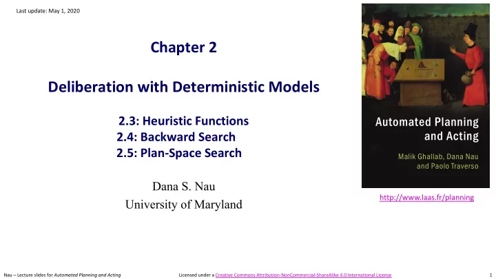
a1 = move(r1,d1,d2)

  • ccupied(d1) = r1

loc(r2) = d1 loc(r1) = d2 loc(r2) = d2 loc(r1) = d1

  • ccupied(d2) = r2
  • ccupied(d3) = nil

ag a0

  • ccupied(d1) = nil
  • ccupied(d2) = r1

loc(r1) = d2

  • ccupied(d2) = nil

loc(r1) = d1 a3 = move(r,d2,d'')

  • ccupied(d'') = nil

loc(r) = d''

  • ccupied(d'') = r
  • ccupied(d2) = nil

loc(r) = d2 a2 = move(r2,d',d1)

  • ccupied(d') = nil
  • ccupied(d1) = r2

loc(r2) = d1

  • ccupied(d1) = nil

loc(r2) = d'

Choosing a Resolver

  • Least Constraining Resolver (LCR):

▸ prefer resolver that rules out the fewest resolvers for the other flaws ≈ Least Constraining Value (LCV) heuristic for CSPs

= Poll: for loc(r)=d2 in a3 , which resolver would

LCR choose first?

1.

causal link from a new action

2.

causal link from a0 , with substitution r←r2

3.

no preference move(r, d, d′) pre: loc(r) = d, occupied(d′) = nil eff: loc(r) ← d′, occupied(d′) = r, occupied(d) = nil

slide-71
SLIDE 71

71 Nau – Lecture slides for Automated Planning and Acting

a1 = move(r1,d1,d2)

  • ccupied(d1) = r1

loc(r2) = d1 loc(r1) = d2 loc(r2) = d2 loc(r1) = d1

  • ccupied(d2) = r2
  • ccupied(d3) = nil

ag a0

  • ccupied(d1) = nil
  • ccupied(d2) = r1

loc(r1) = d2

  • ccupied(d2) = nil

loc(r1) = d1 a3 = move(r,d2,d'')

  • ccupied(d'') = nil

loc(r) = d''

  • ccupied(d'') = r
  • ccupied(d2) = nil

loc(r) = d2 a2 = move(r2,d',d1)

  • ccupied(d') = nil
  • ccupied(d1) = r2

loc(r2) = d1

  • ccupied(d1) = nil

loc(r2) = d'

Choosing a Resolver

  • Least Constraining Resolver (LCR):

▸ prefer resolver that rules out the fewest resolvers for the other flaws ≈ Least Constraining Value (LCV) heuristic for CSPs

  • Problem (in PSP but not in CSPs):

▸ Can keep adding new actions forever Perhaps this might work:

  • Avoid New Actions (ANA) heuristic:

▸ prefer resolvers that don’t add new actions ▸ use LCR as tie-breaker

slide-72
SLIDE 72

72 Nau – Lecture slides for Automated Planning and Acting

a1 = move(r1,d,d2)

  • ccupied(d1) = r1

loc(r2) = d1 loc(r1) = d2 loc(r2) = d2 loc(r1) = d1

  • ccupied(d2) = r2
  • ccupied(d3) = nil

ag a0

  • ccupied(d) = nil
  • ccupied(d2) = r1

loc(r1) = d2

  • ccupied(d2) = nil

loc(r1) = d

  • ccupied(d') = nil
  • ccupied(d1) = r2

loc(r2) = d1

  • ccupied(d1) = nil

loc(r2) = d' a2 = move(r2,d',d1)

Choosing a Resolver

  • Least Constraining Resolver (LCR):

▸ prefer resolver that rules out the fewest resolvers for the other flaws ≈ Least Constraining Value (LCV) heuristic for CSPs

  • Problem (in PSP but not in CSPs):

▸ Can keep adding new actions forever Perhaps this might work:

  • Avoid New Actions (ANA) heuristic:

▸ prefer resolvers that don’t add new actions ▸ use LCR as tie-breaker

= Problem: Ø For loc(r1)=d in a1, ANA chooses a0 with substitution d←d1 Ø For loc(r2)=d′ in a2, ANA chooses a0 with substitution d′←d2 Ø Makes the problem unsolvable = Perhaps use ANA anyway?

slide-73
SLIDE 73

73 Nau – Lecture slides for Automated Planning and Acting

Discussion

  • Problem: how to prune infinitely long paths in the search space?

▸ Loop detection is based on recognizing states

  • r goals we’ve seen before

▸ Partially ordered plan: don’t know the states

  • Prune if π contains the same action more than once?

⟨a1, a2, …, a1, …⟩ ▸ No. Sometimes need the same action again in another state

  • e.g., Towers of Hanoi: move disk1 from peg1 to peg2
  • Weak pruning technique

▸ Prune all partial plans of |S| or more actions ▸ Not very helpful

  • I don’t know whether there’s a better pruning technique

s s' s …

slide-74
SLIDE 74

74 Nau – Lecture slides for Automated Planning and Acting

Summary and Addenda

  • 2.5 Plan-Space Search

▸ Partially ordered plans and solutions ▸ partial plans, causal links ▸ flaws: open goals, threats, resolvers ▸ PSP algorithm, long example, node-selection heuristics ______________________________________________________

  • Two additional sets of lecture slides, if you’re interested

▸ Section 2.7.7, HTN Planning ▸ Section 2.7.8, Planning with Control Rules