CCS 2018 Satellite: DOOCN Thessaloniki 27 September 2018 SIMPLICIAL - PowerPoint PPT Presentation

(a) 80 1 80 1 (b) 0.8 0.8 70 70 0.6 0.6 60 60 0.4 0.4 communities communities 50 50 0.2 0.2 40 0 40 0 -0.2 -0.2 30 30 -0.4 -0.4 20 20 -0.6 -0.6 10 10 -0.8 -0.8 0 0 0 20 40 60 80 0 20 40 60 80 communities communities CCS 2018 Satellite: DOOCN Thessaloniki 27 September 2018 SIMPLICIAL COMPLEXES: EMERGENT HYPERBOLIC NETWORK GEOMETRY AND FRUSTRATED SYNCHRONIZATION Ginestra Bianconi School of Mathema-cal Sciences, Queen Mary University of London, London, UK

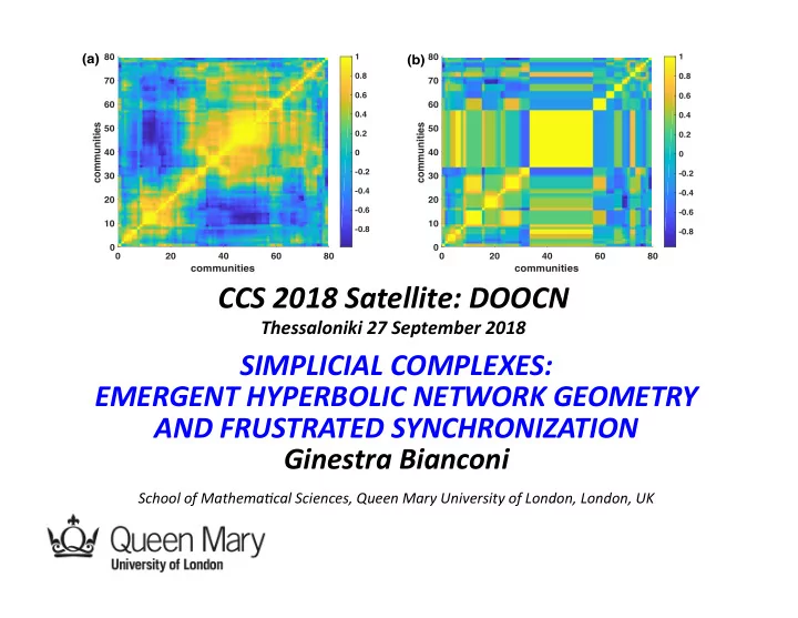
Network Topology and Network Geometry are expected to have impact in a variety of applica3ons, ranging from brain research to rou3ng protocols in the Internet

Community Structure and Network Topology most complex networks have a mesoscale structure which reveal densely connected communi;es From S. Fortunato RMP

The role of dimensionality in neuronal dynamics Uloa Severino et al. Scien3fic Reports (2016)

Generalized network structures Going beyond the framework of simple networks is of fundamental importance for understanding the rela3on between structure and dynamics in complex systems

Simplicial Complexes Simplicial complexes are characterizing the interac3on between two ore more nodes and are formed by nodes, links, triangles, tetrahedra etc. d=2 simplicial complex d=3 simplicial complex

Brain data as simplicial complexes (Gius;, et al 2016) Gius; et al (2016)

Protein interac3on networks as simplicial complexes Protein interac3on networks • Nodes: proteins • Simplices: protein complexes Wan et al. Nature 2015

Collabora3on networks as simplicial complexes Actor collabora;on networks Nodes: Actors • Simplicies: Co-actors of a movie • Scien;fic collabora;on networks Nodes: Scien;sts • Simplicies: Co-authors of a paper •

It is believed that most complex networks have an hidden metric such that the nodes close in the hidden metric are more likely to be linked to each other.

Emergent geometry In the framework of emergent geometry networks with hidden geometry are generated by equilibrium or non-equilibrium dynamics that makes no use of the hidden geometry

Growing networks describe the emergence of scale-free networks Would growing simplicial complexes describe the emergence of hyperbolic complex network geometry?

Generalized degree The generalized degree k d, δ ( µ ) of a δ -face µ in a d-dimensional simplicial complex is given by the number of d-dimensional simplices incident to the δ -face µ . 2 1 Number of triangles k 2 , 0 ( µ ) incident to the node 5 4 µ Number of triangles 3 k 2 , 1 ( µ ) incident to the link µ 6

Generalized degree The generalized degree k d, δ ( µ ) of a δ -face µ in a d-dimensional simplicial complex is given by the number of d-dimensional simplices incident to the δ -face µ . (i,j) k 2,1 ( i , j ) i k 2,0 ( i ) 2 1 (1,2) 1 1 3 (1,3) 3 2 1 (1,4) 1 3 4 5 4 (1,5) 1 4 1 (2,3) 1 5 2 3 (3,4) 1 6 1 (3,5) 2 6 (3,6) 1 (5,6) 1

Incidence number To each (d-1)-face µ we associate the incidence number n µ = k d , d − 1 ( µ ) − 1 (i,j) n ( i , j ) (1,2) 0 2 1 (1,3) 2 (1,4) 0 (1,5) 0 5 4 (2,3) 0 (3,4) 0 3 (3,5) 1 (3,6) 0 6 (5,6) 0

Manifolds If n µ takes only values n µ =0,1 each (d-1)-face is incident at most to two d-dimensional simplices. In this case the simplicial complex is a discrete manifold. 2 1 2 1 5 4 5 3 3 6 6 NOT A MANIFOLD MANIFOLD

Network Geometry with Flavor Starting from a single d-dimensional simplex (1) GROWTH : At every timestep we add a new d simplex (formed by one new node and an existing (d-1)-face). (2) ATTACHMENT : The probability that a new node will be connected to a face µ depends on the flavor s=-1,0,1 and is given by 2 1 1 + sn µ [ s ] = Π µ 5 4 ∑ ( 1 + sn µ ' ) µ ' 3 Bianconi & Rahmede (2016) 6

AVachment probability ⎧ ( 1 − n µ ) , s = − 1 ⎪ Z [ − 1 ] ⎪ ⎪ ( 1 + s n µ ) 1 [ s ] = ⎨ Z [ 0 ] , s = 0 Π µ = ∑ ( 1 + sn µ ' ) ⎪ k µ ⎪ µ ' ∈ Q d , d − 1 Z [ 1 ] , s = 1 ⎪ ⎩ s=-1 Manifold n µ =0,1 s=0 Uniform aVachment n µ =0,1,2,3,4… s=1 Preferen3al aVachment n µ =0,1,2,3,4…

Dimension d=1 Manifold Uniform aVachment Preferen3al aVachment Chain Exponen3al Scale-free BA model

Dimension d=2 Manifold Uniform aVachment Preferen3al aVachment Exponen3al Scale-free Scale-free

Dimension d=3 Manifold Uniform aVachment Preferen3al aVachment Scale-free Scale-free Scale-free

Effec3ve preferen3al aVachment in d=3 t=3 t=4 i i Node i has generalized degree 3 Node i has generalized degree 4 Node i is incident to 5 unsaturated faces Node i is incident to 6 unsaturated faces

Degree distribu3on For d+s=1 k − d ⎛ ⎞ d 1 P d ( k ) = ⎜ ⎟ ⎝ d + 1 ⎠ d + 1 For d+s>1 d ( k ) = d + s Γ ( 1 + ( 2s + s )( d + s − 1 )) Γ ( k − d + d /( d + s − 1 )) P 2d + s Γ ( d /( d + s − 1 )) Γ ( k − d + ( 2d + s )( d + s − 1 )) NGF are always scale-free for d>1-s • For s=1 NGF are always scale free • For s=0 and d>1 the NGF are scale-free • For s=-1 and d>2 the NGF are scale-free

Degree distribu3on of NGF

Generalized degree distribu3ons The power-law generalized degree distribu;on are scale-free for [ δ , s ] = 2( δ + 1) + s d ≥ d c

Emergent community structure Modularity and Clustering coefficient of NGF

Emergent Hyperbolic geometry The emergent hidden geometry is the hyperbolic H d space Here all the links have equal length d=2

Emergent hyperbolic geometry d=3

Apollonian networks are formed by linking the centers of an Apollonian sphere packing They are scale-free and are described by the Lorentz group Andrade et al. PRL 2005 Soderberg PRA 1992

The pseudo-fractal geometry of the surface of the Connec3on with the Apollonian network 3d manifold (random Apollonian network)

Complex Network Manifolds And Frustrated Synchroniza3on

Holography of Complex Network Manifolds d=3 D=2 (a) (b) d-dimensional Complex Network Manifolds can be interpreted as D-dimensional manifolds with D=d-1

Spectral dimensions of Complex Network Manifolds L ij = δ ij − a ij k i ρ c ( λ ) ≈ λ − d s / 2 Complex Network Manifolds have finite spectral dimension with d s ≈ d for d = 2 , 3 , 4

Localiza3on of the eigenvectors The par3cipa3on ra3o evaluates the effec3ve number of nodes on which an eigenmode is localized − 1 ⎡ ⎤ N 2 ∑ ( ) λ v i λ Y λ = u i ⎢ ⎥ ⎣ ⎦ i = 1 A large number of eigenmodes are localized

The Kuramoto model We consider the Kuramoto model N a ij d ϑ i ( ) ∑ sin ϑ j − ϑ i dt = ω i + σ k i j = 1 where ω i is the internal frequency of node i drawn randomly from a Gaussian distribu3on The global order parameter is N R = 1 ∑ i ϑ j e N j = 1

Kuramoto Model In an infinite fully connected network we have R 1 Synchronized phase 0 σ c σ

Frustrated synchroniza3on D=1 D=2 D=3 1.0 1.0 1.0 (a) (b) (c) 0.8 0.8 0.8 R(T) R(T) R(T) 0.6 0.6 0.6 0.4 0.4 0.4 0.2 0.2 0.2 0 0 0 0 5 10 15 0 5 10 15 0 5 10 15 1.0 1.0 1.0 (d) (e) (f) R(t) R(t) R(t) 0.5 0.5 0.5 0 0 0 100 300 500 100 300 500 100 300 500 t t t

Finite size effects D=1 D=2 D=3 1.0 1.0 1.0 (a) (c) (b) 0.8 0.8 0.8 0.6 0.6 0.6 R R R 0.4 0.4 0.4 0.2 0.2 0.2 0 0 0 0 5 10 15 0 5 10 15 5 15 0 10 σ σ σ 0.15 0.15 0.15 (d) (f) (e) 0.10 0.10 0.10 σ R σ R σ R 0.05 0.05 0.05 0 0 0 0 5 10 15 0 5 10 15 σ σ 0 5 σ 10 15 N=100,200,400,800,1600,3200 The finite size effects are less pronounced in larger dimensions

Fully synchronized phase and the spectral dimension The fully synchronized phase is not thermodynamically achieved for networks with spectral dimension d s ≤ 4 In Complex Network Manifolds with D=3 the fully synchronized state is marginally stable

Frustrated synchroniza3on and community structure D=1 D=2 D=3 (a) (b) (c) For every community with n C nodes we can define the local order parameter N Z mod = R mod e i ψ mod = 1 ∑ i ϑ j e n C j ∈ C

Communi3es and Frustrated Synchroniza3on 1.0 1.0 1.0 (a) (b) (c) 0.5 0.5 0.5 Im[Z mod ] Im[Z mod ] Im[Z mod ] 0.0 0.0 0.0 -0.5 -0.5 -0.5 -1.0 -1.0 -1.0 -1.0-0.5 0.0 0.5 1.0 -1.0 -0.5 0.0 0.5 1.0 -1.0-0.5 0.0 0.5 1.0 Re[Z mod ] Re[Z mod ] Re[Z mod ] 1.0 1.0 1.0 R mod (t) R mod (t) R mod (t) 0.5 0.5 0.5 (f) (d) (e) 0.0 0.0 0.0 800 900 1000 800 900 1000 800 900 1000 t t t 300 400 400 (i) (g) (h) 300 300 200 S(f) S(f) S(f) 200 200 100 100 100 0 0-0.4-0.2 0.0 0.2 0-0.4-0.2 0.0 0.2 -0.4-0.2 0.0 0.2 0.4 0.4 0.4 f f f

Localiza3on of eigenvector on communi3es − 1 ⎡ ⎤ 2 ⎛ ⎞ ⎢ ⎥ ∑ ∑ λ v i λ ⎜ ⎟ Y Q = u i ⎜ ⎟ ⎢ ⎥ ⎝ ⎠ ⎣ n i ∈ C n ⎦ measure in how many communi3es the eigenmode is localized D=1 D=2 D=3 1 1 1 (a) (b) (c) 10 -1 10 -1 10 -1 P(Y Q ) P(Y Q ) P(Y Q ) 10 -2 10 -2 10 -2 10 -3 10 -3 10 -3 10 -4 10 -4 10 -4 0 10 20 30 0 5 10 15 20 0 5 10 15 Y Q Y Q Y Q