Call Trees (Tail) Recursion Amtoft from Hatcliff s u m l i s t n - - PowerPoint PPT Presentation

call trees
SMART_READER_LITE
LIVE PREVIEW

Call Trees (Tail) Recursion Amtoft from Hatcliff s u m l i s t n - - PowerPoint PPT Presentation

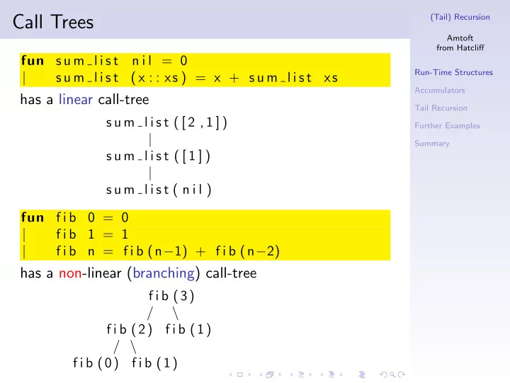
Call Trees (Tail) Recursion Amtoft from Hatcliff s u m l i s t n i l = 0 fun Run-Time Structures | s u m l i s t ( x : : xs ) = x + s u m l i s t xs Accumulators has a linear call-tree Tail Recursion s u m l i s t ( [ 2 , 1 ] )


slide-1
SLIDE 1

(Tail) Recursion Amtoft from Hatcliff Run-Time Structures Accumulators Tail Recursion Further Examples Summary

Call Trees

fun s u m l i s t n i l = 0 | s u m l i s t ( x : : xs ) = x + s u m l i s t xs

has a linear call-tree

s u m l i s t ( [ 2 , 1 ] ) | s u m l i s t ( [ 1 ] ) | s u m l i s t ( n i l ) fun f i b 0 = 0 | f i b 1 = 1 | f i b n = f i b (n−1) + f i b (n−2)

has a non-linear (branching) call-tree

f i b (3) / \ f i b (2) f i b (1) / \ f i b (0) f i b (1)

slide-2
SLIDE 2

(Tail) Recursion Amtoft from Hatcliff Run-Time Structures Accumulators Tail Recursion Further Examples Summary

Stacking Bindings

fun r e v e r s e n i l = n i l | r e v e r s e ( x : : xs ) = r e v e r s e xs @ [ x ] − val L = [ 1 , 2 , 3 ] ; − r e v e r s e (L ) ;

Environment during recursion: (see p. 67)

+ − − − − − − − − − − − − − − − − −+ | | . . added i n r e v e r s e ( n i l ) + − − − − − − − − − − − − − − − − −+ | xs n i l | | x 3 | . . added i n r e v e r s e ( [ 3 ] ) + − − − − − − − − − − − − − − − − −+ | xs [ 3 ] | | x 2 | . . added i n r e v e r s e ( [ 2 , 3 ] ) + − − − − − − − − − − − − − − − − −+ | xs [ 2 , 3 ] | | x 1 | . . added i n r e v e r s e ( [ 1 , 2 , 3 ] ) + − − − − − − − − − − − − − − − − −+ | L [ 1 , 2 , 3 ] | | . . . | . . top l e v e l environment + − − − − − − − − − − − − − − − − −+

slide-3
SLIDE 3

(Tail) Recursion Amtoft from Hatcliff Run-Time Structures Accumulators Tail Recursion Further Examples Summary

Running Time

fun r e v e r s e n i l = n i l | r e v e r s e ( x : : xs ) = ( r e v e r s e xs ) @ [ x ]

◮ Consider calling reverse on a list of length n

◮ it makes n calls to append ◮ which takes time 1, 2, . . . n − 2, n − 1, n

the running time is thus quadratic.

slide-4
SLIDE 4

(Tail) Recursion Amtoft from Hatcliff Run-Time Structures Accumulators Tail Recursion Further Examples Summary

Performance Test

We need generator of large data:

fun from i j = i f i > j then n i l else i : : from ( i +1) j

Execute reverse L where L is the value of (from 1 n) n running time 10,000 2 seconds 20,000 7 seconds 40,000 34 seconds 100,000 very slow When testing sum list, we rather want

fun ones 0 = n i l |

  • nes n = 1

: :

  • nes

(n−1)

slide-5
SLIDE 5

(Tail) Recursion Amtoft from Hatcliff Run-Time Structures Accumulators Tail Recursion Further Examples Summary

Assessment

fun r e v e r s e n i l = n i l | r e v e r s e ( x : : xs ) = ( r e v e r s e xs ) @ [ x ]

Why must we call append?

◮ :: only allows us to add items in front of list ◮ reverse does non-trivial computation only when

going up the tree We might consider doing computation when going down the tree

slide-6
SLIDE 6

(Tail) Recursion Amtoft from Hatcliff Run-Time Structures Accumulators Tail Recursion Further Examples Summary

Passing Results Down In Call Tree

Recall that list reversal is special case of foldl

fun f o l d l f e n i l = e | f o l d l f e ( x : : xs ) = f o l d l f ( f ( x , e )) xs fun my reverse xs = f o l d l

  • p : :

n i l xs ;

Specializing foldl wrt op:: yields

fun r e v a c c e n i l = e | r e v a c c e ( x : : xs ) = r e v a c c ( x : : e ) xs fun r e v e r s e a c c xs = r e v a c c n i l xs

◮ e holds “the results so far” ◮ e is flowing down the tree, informing the recursion at

the next level of something that we have accumulated at the current level

slide-7
SLIDE 7

(Tail) Recursion Amtoft from Hatcliff Run-Time Structures Accumulators Tail Recursion Further Examples Summary

Performance Comparison

◮ Recall that reverse had quadratic running time. ◮ Since reverse acc uses no append, we expect

linear running time. When called on the value of from 1 n n reverse reverse acc 10,000 2 seconds instantaneous 20,000 7 seconds instantaneous 100,000 very slow instantaneous 1,000,000 infeasible 3 seconds

slide-8
SLIDE 8

(Tail) Recursion Amtoft from Hatcliff Run-Time Structures Accumulators Tail Recursion Further Examples Summary

Tail Recursion

fun r e v a c c e n i l = e | r e v a c c e ( x : : xs ) = r e v a c c ( x : : e ) xs

This function is tail recursive:

◮ no computation happens after the recursive call ◮ value of recursive call is the return value ◮ thus, no variables are referenced after recursive call

This kind of recursion is actually iteration in disguise!

slide-9
SLIDE 9

(Tail) Recursion Amtoft from Hatcliff Run-Time Structures Accumulators Tail Recursion Further Examples Summary

Iterative Reverse

fun r e v a c c e n i l = e | r e v a c c e ( x : : xs ) = r e v a c c ( x : : e ) xs

can be converted to “pseudo-C (renaming e to acc):

l i s t r e v e r s e ( xs : l i s t ) { l i s t acc ; acc = [ ] ; while ( xs != n i l ) do { acc = hd ( xs ) : : acc ; xs = t l ( xs ) ; } return acc ; }

◮ acc holds result ◮ xs and acc are updated each time through the loop

slide-10
SLIDE 10

(Tail) Recursion Amtoft from Hatcliff Run-Time Structures Accumulators Tail Recursion Further Examples Summary

Tail Recursion versus Non-Tail Recursion

(∗ v e r s i o n 1: without accumulator ∗) fun r e v e r s e n i l = n i l | r e v e r s e ( x : : xs ) = r e v e r s e xs @ [ x ] (∗ v e r s i o n 2: with accumulator ∗) fun r e v a c c e n i l = e | r e v a c c e ( x : : xs ) = r e v a c c ( x : : e ) xs

x is used after recursion in v.1, but not in v.2

◮ for tail-recursive functions, we do thus not need to

stack variable bindings for the recursive calls

◮ parameter passing can be implemented in the

compiler by destructive updates (that is, assignment)! Computation occurs after recursion in v.1, but not in v.2

◮ for tail-recursive functions, we do thus not need to

stack return addresses; a call can be implemented in the compiler as a goto!

slide-11
SLIDE 11

(Tail) Recursion Amtoft from Hatcliff Run-Time Structures Accumulators Tail Recursion Further Examples Summary

Parameter “Assignment”

The tail-recursive function

fun f ( y 1 , . . . , y n ) = . . . f (<exp −1>, . . . , <exp−n>)

...is roughly equivalent to...

. . . f ( y 1 , . . . , y n ) { while . . . { . . . . . . y 1 = <exp −1>; . . . y n = <exp−n>; } }

slide-12
SLIDE 12

(Tail) Recursion Amtoft from Hatcliff Run-Time Structures Accumulators Tail Recursion Further Examples Summary

Converting SumList to Tail Recursion

fun s u m l i s t n i l = 0 | s u m l i s t ( x : : xs ) = x + s u m l i s t xs

◮ The recursive calls are unfolded until we reach the

end of the list, from where we then move to the left while summing the results.

fun s u m l i s t a c c acc n i l = acc | s u m l i s t a c c acc ( x : : xs ) = s u m l i s t a c c ( x+acc ) xs

◮ Summation proceeds while moving left to right. ◮ Top-level call: sum list acc 0 xs

Performance comparison on the value of ones n n sum list sum list acc 4,000,000 5 seconds instantaneous 5,000,000 21 seconds instantaneous

slide-13
SLIDE 13

(Tail) Recursion Amtoft from Hatcliff Run-Time Structures Accumulators Tail Recursion Further Examples Summary

Tail-Recursive MultList

fun m u l t l i s t a c c acc n i l = acc | m u l t l i s t a c c acc ( x : : xs ) = m u l t l i s t a c c ( x∗ acc ) xs

Question: what happens if we hit a 0?

fun m u l t l i s t a c c e x i t acc n i l = acc | m u l t l i s t a c c e x i t acc ( x : : xs ) = i f x = 0 then 0 else m u l t l i s t a c c e x i t ( x∗ acc ) xs

In C, we might have

i n t m u l t l i s t ( xs : l i s t ) { i n t acc ; acc = 1; while ( xs != n i l ) do { i f ( hd ( xs ) = 0) then return 0; /∗ escape ∗/ e l s e acc = hd ( xs ) ∗ acc ; xs = t l ( xs ) ; } return acc ; }

slide-14
SLIDE 14

(Tail) Recursion Amtoft from Hatcliff Run-Time Structures Accumulators Tail Recursion Further Examples Summary

Making Fibonacci Tail-Recursive

fun f i b 0 = 0 | f i b 1 = 1 | f i b n = f i b (n−2) + f i b (n−1)

has a branching call-tree, and can be made tail-recursive by using two accumulating parameters:

fun f i b a c c prev c u r r n = i f n = 1 then c u r r else f i b a c c c u r r ( prev+c u r r ) (n−1) fun f i b o n a c c i a c c n = i f n = 0 then 0 else f i b a c c 0 1 n

Performance comparison n fib fibonacci acc 42 7 seconds instantaneous 43 11 seconds instantaneous 44 17 seconds instantaneous

slide-15
SLIDE 15

(Tail) Recursion Amtoft from Hatcliff Run-Time Structures Accumulators Tail Recursion Further Examples Summary

Correctness of Tail-Recursive Fibonacci

With F the fibonacci function we have

F(0) = 0; F(1) = 1; F(n) = F(n − 2) + F(n − 1)

which can be tail-recursively implemented by

fun g (n , prev , c u r r ) = i f n = 1 then c u r r else g (n−1, curr , prev+c u r r )

Correctness Lemma: for all n ≥ 1, k ≥ 0: g(n, F(k), F(k + 1)) = F(n + k) This can be proved by induction in n.

◮ the base case is n = 1 which is obvious. ◮ for the inductive case, n > 1,

g(n, F(k), F(k+1)) = g(n−1, F(k+1), F(k)+F(k+1)) = g(n−1, F(k+1), F(k+2)) = F((n−1)+(k+1)) = F(n+k)

Thus F(n) = g(n, F(0), F(1)) = g(n, 0, 1).

slide-16
SLIDE 16

(Tail) Recursion Amtoft from Hatcliff Run-Time Structures Accumulators Tail Recursion Further Examples Summary

Summary

◮ a tail-recursive function is one where the function

performs no computation after the recursive call

◮ a good SML compiler will detect tail-recursive

functions and implement them iteratively

◮ as loops ◮ there is no need to stack bindings or return addresses ◮ recursive calls become gotos ◮ we can think of arguments as being “assigned to”

(destructively update) formal parameters.

◮ this substantially reduces execution time and space

(for stack) overhead