Binary Addition Goals DEF: A binary adder with input length n is a - - PowerPoint PPT Presentation

SLIDE 1

Chapter 6: Addition

Computer Structure - Spring 2004

c

• Dr. Guy Even

Tel-Aviv Univ.

– p.1

Goals

Binary addition - definition Ripple Carry Adder - definition, correctness, cost, delay Carry bits - definition, properties (*) Conditional Sum Adder - definition, correctness, cost, delay (*) Compound Adder - definition, correctness, cost, delay

– p.2

Binary Addition

DEF: A binary adder with input length n is a combinational circuit specified as follows.

Input: A[n − 1 : 0], B[n − 1 : 0] ∈ {0, 1}n, and C[0] ∈ {0, 1}. Output: S[n − 1 : 0] ∈ {0, 1}n and C[n] ∈ {0, 1}. Functionality:

• S + 2n · C[n] =

A + B + C[0]

• A,

B - binary representations of the addends. C[0] - the carry-in bit.

• S - binary representation of the sum.

C[n] - the carry-out bit. Question: is the functionality of ADDER(n) is well defined?

– p.3

Lower bounds

Prove that for every ADDER(n): c(ADDER(n)) = Ω(n) d(ADDER(n)) = Ω(log n)

– p.4

Full Adder

A Full-Adder is a combinational circuit with 3 inputs x, y, z ∈ {0, 1} and 2 outputs c, s ∈ {0, 1} that satisfies: 2c + s = x + y + z. A Full Adder computes a binary representation of the sum of 3 bits. s - called the sum output. c - called the carry-out output. We denote a Full-Adder by FA.

– p.5

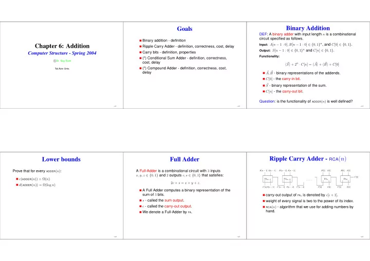
Ripple Carry Adder - RCA(n)

s c fa0 S[0] A[0] B[0] s c fa1 A[1] B[1] C[2] S[1] C[n − 2] s c

fan−2

s c

fan−1

S[n − 2] C[n − 1] S[n − 1] C[n] C[1] A[n − 2] B[n − 2] A[n − 1] B[n − 1] C[0]

carry-out output of FAi is denoted by c[i + 1]. weight of every signal is two to the power of its index.

RCA(n) - algorithm that we use for adding numbers by

hand.

– p.6

SLIDE 2

Correctness proof

To facilitate the proof, we use an equivalent recursive definition of RCA(n). The recursive definition is as follows. Basis: an RCA(1) is simply a Full-Adder. Step:

S[n − 2 : 0] n-1 n-1 n-1 s c

fan−1

S[n − 1] C[n] C[0]

rca(n − 1)

A[n − 1] B[n − 1] C[n − 1] A[n − 2 : 0] B[n − 2 : 0]

– p.7

Correctness - cont.

The proof is by induction on n. The induction basis, for n = 1, follows directly from the defi- nition of a Full-Adder.

– p.8

Induction Step

The induction hypothesis, for n − 1, is (1) A[n − 2 : 0] + B[n − 2 : 0] + C[0] = 2n−1 · C[n − 1] + S[n − 2 : 0]. Full-Adder definition (2) A[n − 1] + B[n − 1] + C[n − 1] = 2 · C[n] + S[n − 1]. Multiply (2) by 2n−1 to obtain (3) 2n−1 · A[n − 1] + 2n−1 · B[n − 1] + 2n−1 · C[n − 1] = 2n · C[n] + 2n−1 · S[n − 1].

– p.9

(1) A[n − 2 : 0] + B[n − 2 : 0] + C[0] = 2n−1 · C[n − 1] + S[n − 2 : 0]. (3) 2n−1 · A[n − 1] + 2n−1 · B[n − 1] + 2n−1 · C[n − 1] = 2n · C[n] + 2n−1 · S[n − 1]. Note that 2n−1 · A[n − 1] + A[n − 2 : 0] = A[n − 1 : 0]. (1) + (3) = ⇒ 2n−1 · C[n − 1] + A[n − 1 : 0] + B[n − 1 : 0] + C[0] = 2n · C[n] + 2n−1 · C[n − 1] + S[n − 1 : 0]. Cancel out 2n−1 · C[n − 1]. QED.

– p.10

Cost & Delay Analysis

The cost of an RCA(n) satisfies: c(RCA(n)) = n · c(FA) = Θ(n). The delay of an RCA(n) satisfies d(RCA(n)) = n · d(FA) = Θ(n).

– p.11

Is RCA(n) good enough?

Clock rate = 1GHz = 109Hz ⇒ clock period = 10−9sec = 1ns. Delay of gate ≈ 100ps = 0.1ns. d(FA) ≈ 2 · d(gate) ≈ 0.2ns. ⇒ Within a clock period we can only add 5-bit numbers... Question: How are > 100 bits added in one clock cycle?

– p.12

SLIDE 3

Carry bits

DEF: The carry bits associated with an addition A + B + C[0] are the signals C[n : 0] in an RCA(n).

s c fa0 S[0] A[0] B[0] s c fa1 A[1] B[1] C[2] S[1] C[n − 2] s c

fan−2

s c

fan−1

S[n − 2] C[n − 1] S[n − 1] C[n] C[1] A[n − 2] B[n − 2] A[n − 1] B[n − 1] C[0]

– p.13

remark 1: redundant & non-redundant representations

Functionality of an adder: A[n − 1 : 0] + B[n − 1 : 0] + C[0] = 2n · C[n] + S[n − 1 : 0]. Let x = A + B + C[0]. x admits two representations (left-hand side, right-hand side) C[n] · S[n − 1 : 0] - binary representation of x. Binary representation is non-redundant: Every value has a unique representation. X = Y ⇐ ⇒ X = Y .

– p.14

remark 1 - cont

Functionality of an adder: A[n − 1 : 0] + B[n − 1 : 0] + C[0] = 2n · C[n] + S[n − 1 : 0]. x = A[n − 1 : 0] + B[n − 1 : 0] + C[0]. many possible combinations of A, B and C[0]. For example: 8 = 4 + 3 + 1, and also 8 = 5 + 3 + 0. → redundant representation. in redundant representation: X = Y = ⇒ value(X) = value(Y ). ⇒ in redundant representation: comparison is complicated.

ADDER(n) - translates a redundant representation to a

non-redundant binary representation.

– p.15

remark 2: cones

The correctness proof of RCA(n) implies that, for every 0 ≤ i ≤ n − 1, A[i : 0] + B[i : 0] + C[0] = 2i+1 · C[i + 1] + S[i : 0]. This equality means that: cone(C[i + 1]), cone(S[i : 0]) ⊆ A[i : 0]

• B[i : 0]
• C[0].

Question: Prove that cone(S[i]), cone(C[i + 1]) = A[i : 0]

• B[i : 0]
• C[0].

– p.16

remark 3

A[i : 0] + B[i : 0] + C[0] = 2i+1 · C[i + 1] + S[i : 0]. = ⇒ for every 0 ≤ i ≤ n − 1, S[i : 0] = mod(A[i : 0] + B[i : 0] + C[0], 2i+1).

– p.17

remark 4: reductions sum-bits ← → carry-bits

The correctness of RCA(n) implies that, for every 0 ≤ i ≤ n − 1, S[i] = XOR(A[i], B[i], C[i]). = ⇒ for every 0 ≤ i ≤ n − 1, C[i] = XOR(A[i], B[i], S[i]). = ⇒ constant-time linear-cost reductions: S[n − 1 : 0] − → C[n − 1 : 0] C[n − 1 : 0] − → S[n − 1 : 0] = ⇒ if Circuit computes C[n − 1 : 0] with O(n) cost and (log n) delay, then we know how to add with same asymptotic cost & delay.

– p.18

SLIDE 4

Chapter 7: Fast Addition: parallel prefix computation

Computer Structure - Spring 2004

c

• Dr. Guy Even

Tel-Aviv Univ.

– p.40

Goals

Design an adder with O(log n) delay and O(n) cost. Learn some interesting methods along the way...

– p.41

reminder: reduction sum-bits − → carry-bits

The correctness of RCA(n) implies that, for every 0 ≤ i ≤ n − 1, S[i] = XOR(A[i], B[i], C[i]). = ⇒ constant-time linear-cost reduction: S[n − 1 : 0] − → C[n − 1 : 0] = ⇒ if Circuit computes C[n−1 : 0] with O(n) cost and O(log n) delay, then we know how to add asymptotically optimally.

– p.42

Computing the carry bits - preliminary

Functionality of Full-Adder (ith FA in RCA(n)): C[i + 1] =

• if A[i] + B[i] + C[i] ≤ 1

1 if A[i] + B[i] + C[i] ≥ 2. Claim: A[i] + B[i] = 0 = ⇒ C[i + 1] = 0 A[i] + B[i] = 2 = ⇒ C[i + 1] = 1 A[i] + B[i] = 1 = ⇒ C[i + 1] = C[i] = ⇒ if A[i] + B[i] ∈ {0, 2}, then easy to compute C[i + 1]. if A[i] + B[i] = 1, then “ripple effect” of carry.

– p.43

definition of σ[n − 1 : −1]

DEF: for i = −1, 0, . . . , n − 1 σ[i]

△

=

• 2 · C[0]

if i = −1 A[i] + B[i] if i ∈ [0, n − 1]. Note that σ[i] ∈ {0, 1, 2}. Claim: for every −1 ≤ i ≤ n − 1, C[i + 1] = 1 ⇐ ⇒ ∃j ≤ i : σ[i : j] = 1i−j · 2.

– p.44

example with σ[n − 1 : −1]

σ[i]

△

=

• 2 · C[0]

if i = −1 A[i] + B[i] if i ∈ [0, n − 1]. Claim: for every −1 ≤ i ≤ n − 1, C[i + 1] = 1 ⇐ ⇒ ∃j ≤ i : σ[i : j] = 1i−j · 2. Example: A[3 : 0] = 0110, B[3 : 0] = 0011, C[0] = 0. position 4 3 2 1

• 1

A 1 1 B 1 1 S 1 1 C 1 1 σ 1 2 1

– p.45

SLIDE 5

Proof: σ[i : j] = 1i−j · 2 ⇒ C[i + 1] = 1

By induction on i − j. Basis i − j = 0: in this case σ[i] = 2. If i = −1, then C[0] = 1. If i ≥ 0, then A[i] + B[i] = 2. Hence C[i + 1] = 1.

• Ind. Step: note that σ[i − 1 : j] = 1i−j−1 · 2.
• Ind. Hyp. ⇒ C[i] = 1.

Since σ[i] = 1, we conclude that A[i] + B[i]

• σ[i]=1

+C[i] = 2. Hence, C[i + 1] = 1.

– p.46

Proof: C[i + 1] = 1 ⇒ ∃j ≤ i : σ[i : j] = 1i−j · 2

By induction on i. Basis i = −1: in this case C[0] = 1, hence σ[−1] = 2. Set j = i.

• Ind. Step: Assume C[i + 1] = 1. Hence,

A[i] + B[i]

• σ[i]

+C[i] ≥ 2. σ[i] = 0: contradiction. σ[i] = 2: set j = i. σ[i] = 1: ⇒ C[i] = 1. C[i] = 1

• Ind. Hyp.

= ⇒ ∃j ≤ i : σ[i − 1 : j] = 1i−j−1 · 2

σ[i]=1

= ⇒ ∃j ≤ i : σ[i : j] = 1i−j · 2.

– p.47

Corollary: method for computing C[i + 1]

C[i + 1] = 1 ⇐ ⇒ ∃j ≤ i : σ[i : j] = 1i−j · 2. Corollary: C[i + 1] =

OR((σ[i : −1] == 1i+1 · 2),

(σ[i : 0] == 1i · 2), (σ[i : 1] == 1i−1 · 2), . . . (σ[i : i − 1] == 1 · 2), (σ[i] == 2) )

– p.48

Carry-Lookahead Generator

C[i + 1] = 1 ⇐ ⇒ ∃j ≤ i : σ[i : j] = 1i−j · 2.

?

= 1 σ[i] · · · · · ·

?

= 1 σ[j + 1]

?

= 2 σ[j] and-tree(i − j + 1) · · · σ[i : j]

?

= 1i−j · 2 σ[i : i − 1]

?

= 1 · 2 σ[i]

?

= 2 · · · σ[i : j]

?

= 1i−j · 2

• r-tree(i + 2)

· · · C[i + 1]

– p.49

Carry-Lookahead Generator: cost & delay

constant cost & depth comparison gates for deciding if : σ[i] = 1 σ[i] = 2 Use a row of comparison gates for σ[i : j]. Feed outputs of comparison gates to AND-tree(i − j + 1). Cost of test σ[i : j] = 1i−j · 2 c(AND-tree(i − j + 1)) + (i − j + 1) · c(comparison) = Θ(i − j). Delay of test σ[i : j] = 1i−j · 2 d(comparison) + (AND-tree(i + j + 1)) = Θ(log(i − j)).

– p.50

Carry-Lookahead Generator: cost & delay - cont.

Test if σ[i : j] = 1i−j · 2 for j = −1, 0, . . . , i. Cost of computing C[i + 1]:

i

• j=−1

c(testing if σ[i : j] = 1i−j · 2) =

i

• j=−1

Θ(i − j) = Θ(i2). Delay of computing C[i + 1]: max

j=−1...i Θ(log(i − j)) = Θ(log i).

⇒ cost of computing C[n : 1]: n−1

i=0 Θ(i2) = Θ(n3).

...usually applied only to short blocks (e.g. 4 bits)

– p.51

SLIDE 6

Carry-Lookahead Adder: typical description

• ✁✂✄

☎ ✆ ✂✝ ✞ ✟ ✠✡ ☛ ✟

• ✂

☞ ✝

• ✌

✂✝ ✄ ✟ ☛✍ ✟ ✎ ✂✏ ✄ ✟ ☎ ✏ ☛ ☛ ✂ ✟

• ✑✓✒

✔ ✕ ✖ ✗ ✘ ✔ ✙ ✔ ✚ ✒ ✔ ✛✜

• ✢

✛

• ✄

✂✄ ✢ ✄ ✂ ☞ ✝ ✣ ✒ ✖ ✗ ✘ ✤ ✙ ✤ ✒ ✤ ✒ ✥ ✗ ✘ ✖ ✙ ✖ ✒ ✖ ✗ ✘ ✖ ✙ ✖ ✘ ✤ ✙ ✖ ✙ ✤ ✒ ✤ ✒ ✦ ✗ ✘ ✥ ✙ ✥ ✒ ✥ ✗ ✘ ✥ ✙ ✥ ✘ ✖ ✙ ✥ ✙ ✖ ✘ ✤ ✙ ✥ ✙ ✖ ✙ ✤ ✒ ✤ ✒ ✧ ✗ ✘ ✦ ✙ ✦ ✘ ✥ ✙ ✦ ✙ ✥ ✘ ✖ ✙ ✦ ✙ ✥ ✙ ✖ ✘ ✤ ✙ ✦ ✙ ✥ ✙ ✖ ✙ ✤ ✒ ✤

from: Introduction to Digital Systems, M.D. Ercegovac, T. Lang, and J.H. Moreno, Wiley and Sons, 1998. – p.52

Carry-Lookahead Adder: typical description

g3 p3 g2

p2

g1 p1 g0 p0 c0 c1 c2 c3 c4 p3 p2 p1 p0

G P CLG-4

from: Introduction to Digital Systems, M.D. Ercegovac, T. Lang, and J.H. Moreno, Wiley and Sons, 1998. – p.53

Carry-Lookahead Adder: typical description

CARRY LOOKAHEAD GENERATOR (CLG-4)

y 0 x 0 c 4 y i x i y 1 x 1 y 2 x 2 y 3 x 3 g2 g1 c 0 G P g3 p 3 p 2 p 1 g0 p 0 p 3 p 2 p 1 p 0 c 3 c 2 c 1 z 3 z 2 z 1 z 0

from: Introduction to Digital Systems, M.D. Ercegovac, T. Lang, and J.H. Moreno, Wiley and Sons, 1998. – p.54

Two-level Carry-Lookahead Adder

2 2 2 2 2 2 2 2 4

z7

4

z6

4

z5

4

z4

4

z3

4

z2

4

z1

4

z0

CLA-4

x7

4 CLA-4

x6

4 CLA-4

x5

4 CLA-4

x4

4 CLA-4

x3

4 CLA-4

x2

4 CLA-4

x1

4 CLA-4

x0

4 G 7 P7 G 6 P6 G 5 P5 G 4 P4 G 3 P3 G 2 P2 G 1 P1 G P0 c4 c8 c12 c20 c24 c28 c32 CLG-4 CLG-4

y7

4

y6

4

y5

4

y4

4

y3

4

y2

4

y1

4

y0

4 c4 c8 c12 c20 c24 c28 c0 c16 c16 carries to CLA-4 modules carries from CLG-4 modules critical path

★✩ ✪ ✫✬ ✭ ✮✯✱✰ ✲ ✳ ✴✵ ✶ ✷✸✹ ✺ ✻✼ ✼ ✽ ✶ ✾ ✿ ✿ ❀ ✻❁ ❂ ✻❃ ✻ ❃ ❃ ❂ ✼ ❄ ❅ ✸❆ ❇ ❈❉ ❊ ❋

• ✻

❆ ❃ ❈❉ ❍ ❋

• ■

✿ ❃ ❄ ✾ ❂ ❅❑❏

from: Introduction to Digital Systems, M.D. Ercegovac, T. Lang, and J.H. Moreno, Wiley and Sons, 1998. – p.55

Definition of ∗ : {0, 1, 2} × {0, 1, 2} − → {0, 1, 2}

∗ 1 2 1 1 2 2 2 2 2 Remark: for every a ∈ {0, 1, 2}: 0 ∗ a = 0 1 ∗ a = a 2 ∗ a = 2. Claim: (homework) ∗ is an associative function. Namely, ∀a, b, c ∈ {0, 1, 2} : (a ∗ b) ∗ c = a ∗ (b ∗ c). Question: Is ∗ commutative?

– p.56

∗-products

For j ≥ i: π[j : i]

△

= σ[j] ∗ · · · ∗ σ[i]. Associativity of ∗ implies that for every i ≤ j < k: π[k : i] = π[k : j + 1] ∗ π[j : i].

– p.57

SLIDE 7

A stronger claim

Claim: For every −1 ≤ i ≤ n − 1, C[i + 1] = 1 ⇐ ⇒ π[i : −1] = 2. Corollary: Can compute C[i + 1] using a ∗-tree(i + 2). ⇒ c(compute C[i + 1]) = O(i) d(compute C[i + 1]) = O(log i). ⇒ c(compute C[n : 1]) =

n

• i=1

O(i) = O(n2) d(compute C[n : 1]) = O(log n). explains carry-lookahead generator... still too expensive!

– p.58

Proof: C[i + 1] = 1 ⇐ ⇒ π[i : −1] = 2

From previous claim, it suffices to prove that ∃j ≤ i : σ[i : j] = 1i−j · 2 ⇐ ⇒ π[i : −1] = 2.

– p.59

Proof: σ[i : j] = 1i−j · 2 ⇒ π[i : −1] = 2

Assume that σ[i : j] = 1i−j · 2. ⇒ π[i : j] = 2. If j = −1 we are done. Otherwise, π[i : −1] = π[i : j]

=2

∗π[j − 1 : −1] = 2.

– p.60

Proof: π[i : −1] = 2 ⇒ ∃j ≤ i : σ[i : j] = 1i−j · 2

Assume that π[i : −1] = 2. If, for every ℓ ≤ i, σ[ℓ] = 2, then π[i : −1] = 2, a

• contradiction. Hence

{ℓ ∈ [−1, i] : σ[ℓ] = 2} = ∅. Let j

△

= max {ℓ ∈ [−1, i] : σ[ℓ] = 2} . π[j : −1] = 2 (since 2 ∗ a = 2). We claim that σ[ℓ] = 1, for every j < ℓ ≤ i.

– p.61

Proof: π[i : −1] = 2 ⇒ ∃j ≤ i : σ[i : j] = 1i−j · 2

Let j

△

= max {ℓ ∈ [−1, i] : σ[ℓ] = 2} . We claim that σ[ℓ] = 1, for every j < ℓ ≤ i.

• max. of j ⇒ for every j < ℓ ≤ i: σ[ℓ] = 2.

if σ[ℓ] = 0, for j < ℓ ≤ i, then π[i : ℓ] = 0. ⇒ π[i : −1] = π[i : ℓ] ∗ π[ℓ − 1 : −1] = 0, a contradiction. since σ[i : j + 1] = 1i−j, we conclude that σ[i : j] = 1i−j · 2, QED.

– p.62

Prefix Computation Problem

DEF: Let Σ denote a finite alphabet. Let OP : Σ2 − → Σ denote an associative function. A prefix computation over Σ with respect to OP is defined as follows.

Input x[n − 1 : 0] ∈ Σn. Output: y[n − 1 : 0] ∈ Σn defined recursively as follows:

y[0] ← x[0] y[i + 1] = OP(x[i + 1], y[i]). Note that y[i] can be also expressed simply by yi = OPi+1(x[i], x[i − 1], . . . , x[0]).

– p.63

SLIDE 8

Reduction: C[n : 1] − → Prefix Computation Prob.

The Claim C[i + 1] = 1 ⇐ ⇒ π[i : −1] = 2 implies a reduction of the problem of computing C[n : 1] to a Prefix Computation Problem: Σ = {0, 1, 2}

OP = ∗

input: σ[−1 : n]

• utput: y[i] = π[i : −1].

– p.64

Prefix Computation Problem - example

Σ = {0, 1}

OP = OR

= ⇒

PPC–OR(n) used to design a Unary Priority Encoder U-PENC(n).

– p.65

Parallel Prefix Circuit

DEF: A Parallel Prefix Circuit, PPC–OP(n), is a combinational circuit that computes a prefix computation. Namely, given input x[n − 1 : 0] ∈ Σn, it outputs y[n − 1 : 0] ∈ Σn, where yi = OPi+1(x[i], x[i − 1], . . . , x[0]). representation of values in Σ - not addressed. assume: some fixed representation is used.

OP-gate: given representations of a, b ∈ Σ, outputs a

representation of OP(a, b).

– p.66

PPC–OP(n) - questions

Question: Design a PPC–OP(n) circuit with linear delay and cost. Question: Design a PPC–OP(n) circuit with logarithmic delay and quadratic cost. Question: Assume that a design C(n) is a PPC–OP(n). This means that it is comprised only of OP-gates and works correctly for every alphabet Σ and associative function

OP : Σ2 → Σ. Can you prove a lower bound on its cost and

delay?

– p.67

PPC–OP - implementation

A recursive design. We already saw a divide-and-conquer design for

PPC–OR(n) with cost Θ(n · log n).

Aim for O(n) cost. “odd-even” divide-and-conquer (as opposed to left/right side divide-and-conquer). basis n = 2: an OP-gate. recursion step...

– p.68

PPC–OP(n) - recursion step

• p-gate
• p-gate
• p-gate
• p-gate
• p-gate
• p-gate
• p-gate

y[0] x[0] x[1] x[2] x[3] x[n − 4] x[n − 3] x[n − 2] x[n − 1] y[1] y[2] y[3] y[n − 4] y[n − 3] y[n − 2] y[n − 1] x′[n/2 − 1] x′[n/2 − 2] x′[1] x′[0] y′[n/2 − 1] y′[n/2 − 2] y′[1] y′[0]

ppc–op(n/2)

– p.69

SLIDE 9

PPC–OP(n) - correctness

By induction. Basis: holds trivially for n = 2. We now prove the induction step. x′[n/2 − 1 : 0], y′[n/2 − 1] - inputs/outputs of PPC–OP(n/2). x′[i] ← OP(x[2i + 1], x[2i]). Induction hypothesis: y′[i] = OPi+1(x′[i], . . . , x′[0]) = OP2i+2(x[2i + 1], . . . , x[0]). y[2i + 1] ← y′[i] ⇒ odd indexed outputs y[1], y[3], . . . , y[n − 1] are correct. y[2i] ← OP(x[2i], y′[i − 1]) = ⇒ y[2i] = OP(x[2i], y[2i − 1]). ⇒ even indexed outputs are also correct. QED

– p.70

PPC–OP(n) - delay analysis (n = 2k)

• p-gate
• p-gate
• p-gate
• p-gate
• p-gate
• p-gate
• p-gate

y[0] x[0] x[1] x[2] x[3] x[n − 4] x[n − 3] x[n − 2] x[n − 1] y[1] y[2] y[3] y[n − 4] y[n − 3] y[n − 2] y[n − 1] x′[n/2 − 1] x′[n/2 − 2] x′[1] x′[0] y′[n/2 − 1] y′[n/2 − 2] y′[1] y′[0]

ppc–op(n/2)

d(PPC–OP(n)) =

• d(OP-gate)

if n = 2 d(PPC–OP(n/2)) + 2 · d(OP-gate)

• therwise.

If follows that d(PPC–OP(n)) = (2 log n − 1) · d(OP-gate).

– p.71

PPC–OP(n) - cost analysis (n = 2k)

• p-gate
• p-gate
• p-gate
• p-gate
• p-gate
• p-gate
• p-gate

y[0] x[0] x[1] x[2] x[3] x[n − 4] x[n − 3] x[n − 2] x[n − 1] y[1] y[2] y[3] y[n − 4] y[n − 3] y[n − 2] y[n − 1] x′[n/2 − 1] x′[n/2 − 2] x′[1] x′[0] y′[n/2 − 1] y′[n/2 − 2] y′[1] y′[0]

ppc–op(n/2)

c(PPC–OP(n)) =

• c(OP-gate)

if n = 2 c(PPC–OP(n/2)) + (n − 1) · c(OP-gate)

• therwise.

It follows that c(PPC–OP(n)) =

k

• i=2

(2i − 1) · c(OP-gate) + c(OP-gate) = (2n − 4 − (k − 1) + 1) · c(OP-gate) = (2n − log n − 2) · c(OP-gate).

– p.72

PPC–OP(n) - corollary

Corollary: If the delay and cost of an OP-gate is constant, then d(PPC–OP(n)) = Θ(log n) c(PPC–OP(n)) = Θ(n). ⇒ Σ = {0, 1} & OP = OR ⇒ asymptotically optimal U-PENC(n). Σ = {0, 1, 2} & OP = ∗ ⇒ compute carry-bits C[n : 1] with O(n) cost and O(log n) delay.

– p.73

PPC–OP(n) - fanout

Insert a buffer in every branching point of the PPC–OP(n) design. ⇒ constant fanout. Question: What is the maximum fanout in the PPC–OP(n)

• design. Analyze the effect of inserting buffers to the

cost and delay of PPC–OP(n).

• p-gate
• p-gate
• p-gate
• p-gate
• p-gate
• p-gate
• p-gate

y[0] x[0] x[1] x[2] x[3] x[n − 4] x[n − 3] x[n − 2] x[n − 1] y[1] y[2] y[3] y[n − 4] y[n − 3] y[n − 2] y[n − 1] x′[n/2 − 1] x′[n/2 − 2] x′[1] x′[0] y′[n/2 − 1] y′[n/2 − 2] y′[1] y′[0]

ppc–op(n/2) – p.74

putting it all together

Compute σ[n − 1 : −1]: Cost & delay are constant per σ[i]. ⇒ total cost is O(n) & the total delay is O(1).

PPC– ∗ (n): Compute product π[i : −1] from σ[i : −1], for

every i ∈ [n − 1 : 0]. The cost O(n) and delay O(log n). Extraction of C[n : 1]: Recall C[i + 1] = 1 iff π[i : −1] = 2. Compare each π[i : −1] with 2. The result of this comparison equals C[i + 1]. The cost and delay is constant per carry-bit C[i + 1]. Total cost of this step is O(n) and the delay is O(1). Computation of sum-bits: The sum bits are computed by S[i] = XOR3(A[i], B[i], C[i]). Cost of this step is O(n) and the delay is O(1).

– p.75

SLIDE 10

Fast Addition

By combining the cost and delay of each stage we obtain the following result. Theorem: The adder based on parallel prefix computation is asymptotically optimal; its cost is linear and its delay is logarithmic.

– p.76

Summary

Presented an adder with asymptotically optimal cost and delay. Design based on two reductions: reduction of the task of computing the sum-bits to the task of computing the carry bits. reduction of the task of computing the carry bits to a prefix computation problem. A prefix computation problem is the problem of computing OPi(x[i − 1 : 0]), for 0 ≤ i ≤ n − 1, where OP is an associative operation.

PPC–OP(n) - a linear cost logarithmic delay circuit for the

prefix computation problem. Can use PPC–OP(n) for asymptotically optimal U-PENC(n).

– p.77