Beyond binary classification Theory and programming Due Wednesday, - PowerPoint PPT Presentation

Administrivia Mini-project 1 posted ! ‣ One of three ‣ Decision trees and perceptrons Beyond binary classification ‣ Theory and programming ‣ Due Wednesday, March 04, 11:55pm 4:00pm ➡ Turn in a hard copy in the CS office Subhransu Maji ‣ Must be done individually, but feel free to discuss with others CMPSCI 689: Machine Learning ‣ Start early … 19 February 2015 CMPSCI 689 Subhransu Maji (UMASS) 2 /27 Today’s lecture Learning with imbalanced data Learning with imbalanced data ! 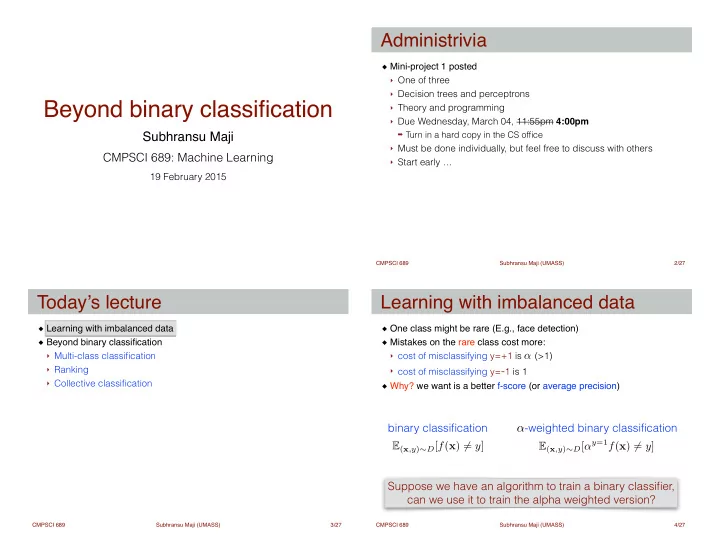One class might be rare (E.g., face detection) ! Beyond binary classification ! Mistakes on the rare class cost more: ! ‣ Multi-class classification ‣ cost of misclassifying y=+1 is (>1) α ‣ Ranking ‣ cost of misclassifying y= - 1 is 1 ‣ Collective classification Why? we want is a better f-score (or average precision) binary classification -weighted binary classification α E ( x ,y ) ∼ D [ α y =1 f ( x ) 6 = y ] E ( x ,y ) ∼ D [ f ( x ) 6 = y ] Suppose we have an algorithm to train a binary classifier, can we use it to train the alpha weighted version? CMPSCI 689 Subhransu Maji (UMASS) 3 /27 CMPSCI 689 Subhransu Maji (UMASS) 4 /27

Training by sub-sampling Proof of the claim Error on D = E ( x ,y ) ∼ D [ ` α (ˆ y, y )] D α Input: Output: ! D, α X = ( D ( x , +1) ↵ [ˆ y 6 = 1] + D ( x , � 1)[ˆ y 6 = � 1]) ! x While true ! X ◆! We have sub-sampled the ✓ y 6 = 1] + 1 ( x , y ) ∼ D ‣ Sample = ↵ D ( x , +1)[ˆ ↵ D ( x , � 1)[ˆ y 6 = � 1] negatives by t ∼ uniform(0 , 1) ‣ Sample x y > 0 or t < 1 / α ‣ If X ! = ↵ ( D α ( x , +1)[ˆ y 6 = 1] + D α ( x , � 1)[ˆ y 6 = � 1]) ➡ return ( x , y ) x sub-sampling algorithm = ↵✏ Claim binary classification -weighted binary classification binary classification -weighted binary classification α α D α D D α D ✏ ↵✏ ✏ ↵✏ CMPSCI 689 Subhransu Maji (UMASS) 5 /27 CMPSCI 689 Subhransu Maji (UMASS) 6 /27 Modifying training Overview To train simply — ! Learning with imbalanced data ! ‣ Subsample negatives and train a binary classifier. Beyond binary classification ! ‣ Alternatively, supersample positives and train a binary classifier. ‣ Multi-class classification ‣ Which one is better? ‣ Ranking ‣ Collective classification For some learners we don’t need to keep copies of the positives ! ‣ Decision tree ➡ Modify accuracy to the weighted version ‣ kNN classifier ➡ Take weighted votes during prediction ‣ Perceptron? CMPSCI 689 Subhransu Maji (UMASS) 7 /27 CMPSCI 689 Subhransu Maji (UMASS) 8 /27

Multi-class classification One-vs-all (OVA) classifier Labels are one of K different ones. ! Train K classifiers, each to distinguish one class from the rest ! Some classifiers are inherently multi-class — ! Prediction: pick the class with the highest score: ! ‣ kNN classifiers: vote among the K labels, pick the one with the ! highest vote (break ties arbitrarily) i ← arg max f i ( x ) score function ! ‣ Decision trees: use multi-class histograms to determine the best ! feature to splits. At the leaves predict the most frequent label. Example ! Question: can we take a binary classifier and turn it into multi-class? i ← arg max w T ‣ Perceptron : i x ➡ May have to calibrate the weights (e.g., fix the norm to 1) since we are comparing the scores of classifiers ➡ In practice, doing this right is tricky when there are a large number of classes CMPSCI 689 Subhransu Maji (UMASS) 9 /27 CMPSCI 689 Subhransu Maji (UMASS) 10 /27 One-vs-one (OVO) classifier Directed acyclic graph (DAG) classifier DAG SVM [Platt et al., NIPS 2000] ! Train K(K-1)/2 classifiers, each to distinguish one class from another ! ‣ Faster testing: O(K) instead of O(K(K-1)/2) Each classifier votes for the winning class in a pair ! ‣ Has some theoretical guarantees The class with most votes wins ! ! 0 1 ! @X f ji = − f ij i ← arg max f ij ( x ) A ! j ! ! 0 1 Example ! @X � w T � ‣ Perceptron : i ← arg max sign ij x A w ji = − w ij ! j ➡ Calibration is not an issue since we are taking the sign of the score Figure from Platt et al. CMPSCI 689 Subhransu Maji (UMASS) 11 /27 CMPSCI 689 Subhransu Maji (UMASS) 12 /27

Overview Ranking Learning with imbalanced data ! Beyond binary classification ! ‣ Multi-class classification ‣ Ranking ‣ Collective classification CMPSCI 689 Subhransu Maji (UMASS) 13 /27 CMPSCI 689 Subhransu Maji (UMASS) 14 /27 Ranking Learning to rank Input: query (e.g. “cats”) ! For simplicity lets assume we are learning to rank for a given query. ! Output: a sorted list of items ! Learning to rank: ! ‣ Input: a list of items ! How should we measure performance? ! ‣ Output: a function that takes a set of items and returns a sorted list The loss function is trickier than in the binary classification case ! ! ‣ Example 1: All items in the first page should be relevant ! ‣ Example 2: All relevant items should be ahead of irrelevant items Approaches ! ‣ Pointwise approach: ➡ Assumes that each document has a numerical score. ➡ Learn a model to predict the score (e.g. linear regression). ‣ Pairwise approach: ➡ Ranking is approximated by a classification problem. ➡ Learn a binary classifier that can tell which item is better given a pair. CMPSCI 689 Subhransu Maji (UMASS) 15 /27 CMPSCI 689 Subhransu Maji (UMASS) 16 /27

Naive rank train Problems with naive ranking Create a dataset with binary labels ! features for Naive rank train works well for bipartite ranking problems ! ‣ Initialize: D ← φ x ij comparing ‣ Where the goal is to predict whether an item is relevant or not. ‣ For every i and j such that, i ≠ j item i and j There is no notion of an item being more relevant than another. ➡ If item i is more relevant than j A better strategy is to account for the positions of the items in the list ! D ← D ∪ ( x ij , +1) • Add a positive point: Denote a ranking by: ! σ ➡ If item i is less relevant than j ‣ If item u appears before item v, we have: σ u < σ v D ← D ∪ ( x ij , − 1) • Add a negative point: Σ M Let the space of all permutations of M objects be: ! Learn a binary classifier on D ! f : X → Σ M A ranking function maps M items to a permutation: ! Ranking ! A cost function (omega) ! ‣ Initialize: score ← [0 , 0 , . . . , 0] ‣ The cost of placing an item at position i at j: ω ( i, j ) ‣ For every i and j such that, i ≠ j Ranking loss: X ` ( � , ˆ � ) = [ � u < � v ][ˆ � v < ˆ � u ] ! ( u, v ) ➡ Calculate prediction: y ← f (ˆ x ij ) u 6 = v ➡ Update scores: score i = score i + y score j = score j − y ! -ranking: min E ( X , σ ) ∼ D [ ` ( � , ˆ � )] , where ˆ � = f ( X ) ranking ← arg sort ( score ) f CMPSCI 689 Subhransu Maji (UMASS) 17 /27 CMPSCI 689 Subhransu Maji (UMASS) 18 /27 ω -rank loss functions ω -rank train Create a dataset with binary labels ! To be a valid loss function ω must be: ! features for D ← φ ‣ Initialize: x ij comparing ‣ Symmetric: ω ( i, j ) = ω ( j, i ) item i and j ‣ For every i and j such that, i ≠ j ω ( i, j ) ≤ ω ( i, k ) if i < j < k or k < j < i ‣ Monotonic: ➡ If σ ᵢ < σ ⱼ (item i is more relevant) ω ( i, j ) + ω ( j, k ) ≥ ω ( i, k ) ‣ Satisfy triangle inequality: D ← D ∪ ( x ij , +1 , ω ( i, j )) • Add a positive point: ! ➡ If σ ᵢ > σ ⱼ (item j is more relevant) Examples: ! D ← D ∪ ( x ij , − 1 , ω ( i, j )) • Add a negative point: ‣ Kemeny loss: Learn a binary classifier on D (each instance has a weight) ! ! ω ( i, j ) = 1, for i 6 = j Ranking ! ! score ← [0 , 0 , . . . , 0] ‣ Initialize: ‣ Top-K loss: ⇢ 1 if min( i, j )  K, i 6 = j ‣ For every i and j such that, i ≠ j ω ( i, j ) = 0 otherwise y ← f (ˆ ➡ Calculate prediction: x ij ) ➡ Update scores: score i = score i + y score j = score j − y ranking ← arg sort ( score ) CMPSCI 689 Subhransu Maji (UMASS) 19 /27 CMPSCI 689 Subhransu Maji (UMASS) 20 /27

Overview Collective classification Predicting multiple correlated variables Learning with imbalanced data ! Beyond binary classification ! ‣ Multi-class classification ‣ Ranking ‣ Collective classification input output ( x , k ) ∈ X × [ K ] G ( X , k ) be the set of all graphs features labels objective f : G ( X ) → G ([ K ]) E ( V,E ) ∼ D [ Σ v ∈ V (ˆ y v 6 = y v )] CMPSCI 689 Subhransu Maji (UMASS) 21 /27 CMPSCI 689 Subhransu Maji (UMASS) 22 /27 Collective classification Stacking classifiers Predicting multiple correlated variables Train a two classifiers ! First one is trained to predict output from the input ! Second is trained on the input and the output of first classifier y (1) ˆ ← f 1 ( x v ) y v ← f ( x v ) ˆ v independent predictions can be noisy x v ← [ x v , φ ([ K ] , nbhd( v ))] labels of ⇣ ⇣ ⌘⌘ y (2) y (1) nearby vertices ˆ ← f 2 x v , φ ˆ v , nbhd( v ) v as features E.g., histogram of labels in a 5x5 neighborhood CMPSCI 689 Subhransu Maji (UMASS) 23 /27 CMPSCI 689 Subhransu Maji (UMASS) 24 /27