Auto tomat mated d Pla lanning ing State + action unique - - PowerPoint PPT Presentation

jonas.kvarnstrom@liu.se – 2020

Auto tomat mated d Pla lanning ing

Planni ning ngunder Uncert rtainty nty

Jonas Kvarnström Department of Computer and Information Science Linköping University

2

jonkv@ida jonkv@ida

2

Multiple iple Outcome comes

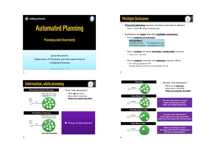
 Classical planning assumes we know outcomes in advance ▪ State + action ➔ unique resulting state  Sometimes we must deal with multiple outcomes ▪ Due to problems in execution ▪ Intended outcome: is true Unintended outcome: is false ▪ Due to random but clearly desirable / undesirable outcomes ▪ Toss a coin – do I win? ▪ Due to random outcomes with unknown long term effects ▪ Do I end up in group A or B? No idea which one will turn out to be better for me

3

jonkv@ida jonkv@ida

3

Infor

• rmation,

mation, while le planning ing

 First ”info dimension”: ▪ What do we know about action outcomes when we create the plan?

Start here… Model says: we end up in one of these states

Non-Deterministic Planning Probabilistic Planning

 Focus of this lecture!

Start here…

0.1 0.2 .07 0.1 .03

Model says: we end up in one of these states …with this probability

 Second ”info dimension”: ▪ What do we find out about action outcomes when we execute the plan? Planning Non-Observable Partially Observable Fully Observable No new information sensed after executing an action Only our initial predictions Can get some information Some aspects are not observable Still uncertain about the current state After executing an action we know the state we ended up in  Focus of this lecture!

1 2 3 4

6

jonkv@ida jonkv@ida

6

State te Transi sition tion Syste tem

 Classical planning: A state transition system Σ = (𝑇, 𝐵, 𝛿) ▪ 𝑇 Finite set of world states ▪ 𝐵 Finite set of actions ▪ 𝛿 × → State transition function, specifying all “edges”

7

jonkv@ida jonkv@ida

7

Stoch chas astic tic Syste tem

 Probabilistic planning uses a stochastic system Σ = (𝑇, 𝐵, 𝑄) ▪ Finite set of world states ▪ Finite set of actions ▪ Given that we are in s and execute a, the probability of ending up in s’

Start here…

0.1 0.2 .07 0.1 .03

Model says: we end up in one of these states

Planning

…with this probability

Replaces 

8

jonkv@ida jonkv@ida

8

Stoch chas astic tic Syste tems ms (2)

At location 5 At location 6 Intermediate location Action: drive-uphill Model says: 2% risk

• f slipping, ending up

somewhere else

Arc indicates

• utcomes of a

single action

Example with "desirable outcome"

5 6 7 8

9

jonkv@ida jonkv@ida

9

Stoch chas astic tic Syste tems ms (3)

 May have very unlikely outcomes… At location 5 At location 6 Intermediate location Broken Very unlikely outcome, but may still be important to consider, if it has great impact on goal achievement!

10

jonkv@ida jonkv@ida

10

Stoch chas astic tic Syste tems ms (4)

 As always, can have many executable actions in a state Probability = 1 (certain outcome) Probability sum = 1 (three possible

• utcomes of A2)

Probability sum = 1 (four possible

• utcomes of A3)

The planner chooses the action to execute… Suppose we choose green. Nature chooses the outcome, so we must be prepared for all 4 green outcomes! Directly searching the state space yields an AND/OR tree 3 possible actions (red, blue, green) Arcs connect edges belonging to the same action

Important concepts, before we define the planning problem itself!

12

jonkv@ida jonkv@ida

12

Stoch chas astic tic Syste tem Exam ample ple

 Example: A single robot ▪ Moving between locations ▪ For simplicity, states correspond directly to locations ▪ ▪ ▪ ▪ ▪ ▪ Some transitions are deterministic, some are stochastic ▪ Trying to move from to : You may end up at instead ( % risk) ▪ Trying to move from to : You may stay where you are instead ( % risk)

wait wait wait wait

s2 s3 s4 s1 s5

move(l2,l3 l3) move(l3,l2 l2) move(l4,l1) move(l1,l4 l4) move(l2,l1 l1) move(l1,l2 l2) move(l4,l3) move(l3,l4 l4) move(l5,l4 l4) wait

9 10 11 12

13

jonkv@ida jonkv@ida

13

Polic icies; ies; Example mple 1

 One type of formal plan structure: Policy 𝜌 ∶ 𝑇 → 𝐵 ▪ Defining, for each state, which action to execute whenever we are there ▪ Possible due to full observability!  Example

▪ Start wait wait wait wait

s2 s3 s4 s1 s5

move(l2,l3 l3) move(l3,l2 l2) move(l4,l1) move(l1,l4 l4) move(l2,l1 l1) move(l1,l2 l2) move(l4,l3) move(l3,l4 l4) move(l5,l4 l4) wait

Reaches

• r

, waits there infinitely many times

14

jonkv@ida jonkv@ida

14

Polic icy y Example mple 2

 Example

▪ Start wait wait wait wait

s2 s3 s4 s1 s5

move(l2,l3 l3) move(l3,l2 l2) move(l4,l1) move(l1,l4 l4) move(l2,l1 l1) move(l1,l2 l2) move(l4,l3) move(l3,l4 l4) move(l5,l4 l4) wait

Always reaches state , waits there infinitely many times

15

jonkv@ida jonkv@ida

15

Polic icy y Example mple 3

 Example

▪ Start wait wait wait wait

s2 s3 s4 s1 s5

move(l2,l3 l3) move(l3,l2 l2) move(l4,l1) move(l1,l4 l4) move(l2,l1 l1) move(l1,l2 l2) move(l4,l3) move(l3,l4 l4) move(l5,l4 l4) wait

Reaches state with % probability ”in the limit” (the more steps, the greater the probability)

16

jonkv@ida jonkv@ida

16

Polic icies ies and Histor tories ies

 The outcome of sequentially executing a policy: ▪ A state sequence   called a history ▪ Infinite, since policies have no termination criterion  For each policy, there can be many potential histories ▪ Which one is the actual result? Gradually discovered at execution time!

13 14 15 16

17

jonkv@ida jonkv@ida

17

Histor tory y Example mple

 Example 1

▪

 Even if we only consider starting in

: Two possible histories

▪

  – Reached , waits indefinitely   – Reached , waits indefinitely

Start wait wait wait wait

s2 s3 s4 s1 s5

move(l2,l3 l3) move(l3,l2 l2) move(l4,l1) move(l1,l4 l4) move(l2,l1 l1) move(l1,l2 l2) move(l4,l3) move(l3,l4 l4) move(l5,l4 l4) wait

How probable are these histories?

18

jonkv@ida jonkv@ida

18

Probabili abilitie ties: Initia tial l State tes, s, Transi sitions tions

 Each policy has a probability distribution over histories/outcomes ▪ With known fixed initial state 𝑡0:

𝑄 𝒕𝟏,𝒕𝟐, 𝒕𝟑, 𝒕𝟒, …  𝜌 = ෑ

𝑗≥0

𝑄(𝑡𝑗, 𝜌 𝑡𝑗 , 𝑡𝑗+1)

▪ With unknown initial state:

𝑄(〈𝒕𝟏, 𝒕𝟐, 𝒕𝟑, 𝒕𝟒, …  | 𝜌) = 𝑄 𝑡0 ⋅ ෑ

𝑗≥0

𝑄(𝑡𝑗, 𝜌 𝑡𝑗 , 𝑡𝑗+1)

Start wait wait wait wait

s2 s3 s4 s1 s5

move(l2,l3) 3) move(l3, 3,l2) move(l4,l1) move(l1,l4) move(l2,l1) move(l1,l2) move(l4,l3) 3) move(l3, 3,l4) move(l5, 5,l4) wait

Probability

• f starting in

this specific 𝑡0 Probabilities for each required state transition

19

jonkv@ida jonkv@ida

19

Histor tory y Example mple 1

 Example

▪

 Two possible histories, if 𝑄 𝑡1 = 1: ▪             

Start wait wait wait wait

s2 s3 s4 s1 s5

move(l2,l3 l3) move(l3,l2 l2) move(l4,l1) move(l1,l4 l4) move(l2,l1 l1) move(l1,l2 l2) move(l4,l3) move(l3,l4 l4) move(l5,l4 l4) wait

20

jonkv@ida jonkv@ida

20

Histor tory y Example mple 2

 Example

▪

▪

            

Start wait wait wait wait

s2 s3 s4 s1 s5

move(l2,l3 l3) move(l3,l2 l2) move(l4,l1) move(l1,l4 l4) move(l2,l1 l1) move(l1,l2 l2) move(l4,l3) move(l3,l4 l4) move(l5,l4 l4) wait

17 18 19 20

21

jonkv@ida jonkv@ida

21

Histor tory y Example mple 3

 Example

▪

▪

                      

∞

    

Start wait wait wait wait

s2 s3 s4 s1 s5

move(l2,l3 l3) move(l3,l2 l2) move(l4,l1) move(l1,l4 l4) move(l2,l1 l1) move(l1,l2 l2) move(l4,l3) move(l3,l4 l4) move(l5,l4 l4) wait

23

jonkv@ida jonkv@ida

23

Stoch chas astic tic Shorte test st Path h Proble lem

 Closest to classical : Stochastic Shortest Path Problem ▪ Let  = (𝑇, 𝐵, 𝑄) be a stochastic system ▪ Let 𝑑: 𝑇, 𝐵 → 𝑆 be a cost function ▪ Let 𝑡0 ∈ 𝑇 be an initial state ▪ Let 𝑇𝑕 ⊆ 𝑇 be a set of goal states ▪ Then, find a policy that can be applied starting at and that reaches a state in Not covered here

21 22 23 24

25

jonkv@ida jonkv@ida

25

Generalizati ralizatingfrom the SSPP

 Policies allow indefinite execution ▪ No predetermined termination criterion – go on "forever” ▪ 𝜌 𝜌 𝑡  Combination of: ▪ Cost function 𝑑(𝑡, 𝑏) ▪ Cost of being in state 𝑡 and executing action 𝑏 ▪ Reward function 𝑆 𝑡, 𝑏, 𝑡′ ▪ Reward for being in state 𝑡, executing action 𝑏 and actually ending up in 𝑡′ But without goal states, what is the objective? What is a good policy?

26

jonkv@ida jonkv@ida

26

Example mple: Grid World ld

 Example: Grid World ▪ Actions: North, South, West, East, NorthWest, …, TakeGold ▪ Cost 𝑑(𝑡, 𝑏) = 10 for all 𝑡, 𝑏 ▪ 90% chance: Go where you want ▪ 10% risk: End up somewhere else ▪ Rewards for some transitions ▪ 𝑆 𝑡, 𝑏, 𝑡′ = +100 for transitions when you take the gold in the top right cell ▪ s = [top right, there is gold] a = TakeGold s’ = [top right, there is no gold] ▪ Danger in some cells ▪ Try to go to the top right cell ▪ 𝑆 𝑡, 𝑏, 𝑡′ = 0 usually ▪ 𝑆 𝑡, 𝑏, 𝑡′ = −200 if you accidentally end up in the danger cell

• 100
• 200

+100

• 80

+50

Important: States != locations Can’t take the gold twice, can’t gain infinite rewards

27

jonkv@ida jonkv@ida

27

Example mple: Tetr tris is

▪ In each ”step”, a piece falls one row – and you execute one action ▪ Guide the pieces left/right, rotate them, drop them ▪ If an action/step results in filling a row: ▪ The line disappears ▪ 𝑆 𝑝𝑚𝑒 𝑡𝑢𝑏𝑢𝑓, 𝑏𝑑𝑢𝑗𝑝𝑜, 𝑡𝑢𝑏𝑢𝑓 𝑥𝑗𝑢ℎ 𝑠𝑝𝑥 𝑠𝑓𝑛𝑝𝑤𝑓𝑒 = 100 ▪ If an action/step results in filling two rows: ▪ 𝑆 𝑝𝑚𝑒 𝑡𝑢𝑏𝑢𝑓, 𝑏𝑑𝑢𝑗𝑝𝑜, 𝑡𝑢𝑏𝑢𝑓 𝑥𝑗𝑢ℎ 2 𝑠𝑝𝑥𝑡 𝑠𝑓𝑛𝑝𝑤𝑓𝑒 = 400 ▪ When a piece has fallen all the way: ▪ A new random piece falls from the top ▪ Model piece probabilities using 𝑄 𝑡, 𝑏, 𝑡′ according to (most types of) Tetris rules

28

jonkv@ida jonkv@ida

28

Example mple: Robot

• t Navig

igati ation

• n

 Example costs in robot navigation: ▪ 𝑑(𝑡, 𝑏) = 1 ▪ 𝑑(𝑡, 𝑏) = 100 ▪ 𝑑(𝑡, 𝑥𝑏𝑗𝑢) = 1

c=1 c=1 c=1 c=1

s2 s2 s3 s3 s4 s4 s1 s1 s5 s5

c=1 c=1 c=1 c=1 c=100 c=100 c=100 c=100 c=100

25 26 27 28

29

jonkv@ida jonkv@ida

29

Example mple: Robot

• t Navig

igati ation

• n (2)

 Example rewards in robot navigation ▪ Every time you end up in s5: ▪ Negative reward – maybe the robot is in our way ▪ Every time you end up in s4: ▪ Positive reward – maybe it helps us

c=1 c=1 c=1 c=1 c=0 c=0 c=0 c=0

s2 s2 s3 s3 s4 s4 s1 s1 s5 s5

c=1 c=1 c=1 c=1 c=1 c=1 c=1 c=1 c=100 c=100 c=100 c=100 c=100

r=0 r=0 r=0 r=0 r=0 r=0 r= r= –100 100 r=+100 00

30

jonkv@ida jonkv@ida

30

Simplif lific icati ation

• n

 To simplify formulas, include the cost in the reward! ▪ Decrease each 𝑆(𝑡𝑗, 𝜌(𝑡𝑗), 𝑡𝑗+1) by 𝐷(𝑡𝑗, 𝜌(𝑡𝑗))

r= -1 r= -1 r= -100 100 r= 100

s2 s2 s3 s3 s4 s4 s1 s1 s5 s5

r= -1 r= 99 r= -100 100 r= -100 100 r= 0 r= -100 100 r= -200 r= -1

How useful is an outcome to us?

32

jonkv@ida jonkv@ida

32

Total al Reward ards s –In Advance ance?

 Given a policy 𝜌, what will our total rewards be? ▪ Can’t know in advance ▪ Will I reach the goal or end up in the danger zone? ▪ Which pieces will I get?

• 100
• 200

+100

• 80

+50

29 30 31 32

33

jonkv@ida jonkv@ida

33

Total al Reward ards s –After r Executing? cuting?

 Given a policy 𝜌… ▪ …and an outcome, an infinite history (state sequence) ℎ = 〈𝑡0, 𝑡1, 𝑡2, … 〉 resulting from actually having executed 𝜌…  …What were our total rewards? ▪ Undiscounted utility of a history: V ℎ 𝜌 = ෍

𝑗≥0

𝑆 𝑡𝑗, 𝜌 𝑡𝑗 , 𝑡𝑗+1

▪ I was in 𝑡0, executed 𝜌 𝑡0 , and ended up in 𝑡1 -- reward! ▪ I was in 𝑡1, executed 𝜌 𝑡1 , and ended up in 𝑡2 −− reward! ▪ I was in 𝑡2, executed 𝜌 𝑡2 , and ended up in 𝑡3 −− reward! ▪ …

35

jonkv@ida jonkv@ida

35

Utilit lityin a Conte text

Policy = solution for infinite horizon We will stop at some point (the universe will end), but we can't predict when To find the best policy for long term execution: Consider the infinite case Indefinite execution Never ends – unrealistic (Infinite actual execution)

36

jonkv@ida jonkv@ida

36

Infinite inite Undis iscoun counte ted Utilit lity

 If we use undiscounted utility for an infinite history: ▪ 𝜌1 could result in   ▪ Stays at forever, executing “wait” ➔ infinite amount of rewards! ▪

r= -1 r= -1 r= -100 100 r= 100

s2 s2 s3 s3 s4 s4 s1 s1 s5 s5

r= -1 r= 99 r= -100 100 r= -100 100 r= 0 r= -100 100 r= -200 r= -1

33 34 35 36

37

jonkv@ida jonkv@ida

37

Infinite inite Undis iscoun counte ted Utilit lity (2)

 What’s the problem, if we "like" being in state

?

▪ Can’t distinguish between different ways of getting there! ▪ → → →   ▪ → → → → →   ▪ Both appear equally good… ▪ Can’t distinguish between

infinite times 100 and and infinite times 1000

▪ Even without infinity,

we can’t see the difference between rewards now and rewards in the far future

r= -1 r= -1 r= -100 100 r= 100

s2 s2 s3 s3 s4 s4 s1 s1 s5 s5

r= -1 r= 99 r= -100 100 r= -100 100 r= 0 r= -100 100 r= -200 r= -1

38

jonkv@ida jonkv@ida

38

Disc scou

• unte

ted Utilit lity

 Solution: Discounted utility for a history ▪ Introduce a discount factor, , with 0 ≤  ≤ 1 ▪ Let 𝑊 ℎ 𝜌 = ෍

𝑗≥0

𝛿𝑗 𝑆(𝑡𝑗, 𝜌 𝑡𝑗 , 𝑡𝑗+1)

▪ Distant rewards/costs

have less influence

▪ For example: 0.9, 0.81, 0.729, … ▪ Convergence (finite results)

is guaranteed if 0 ≤ 𝛿 < 1

Examples will use 𝛿 = 0.9 Only to simplify formulas! Should choose carefully…

r= -1 r= -1 r= -100 100 r= 100

s2 s2 s3 s3 s4 s4 s1 s1 s5 s5

r= -1 r= 99 r= -100 100 r= -100 100 r= 0 r= -100 100 r= -200 r= -1

40

jonkv@ida jonkv@ida

40

Expe pecte cted Utility ity of a Polic icy

 We want to choose a good policy ▪ We know, for each history (outcome)   of a policy 𝜌: ▪ The probability that the history will occur: 𝑄 ℎ 𝜌 ▪ The resulting actual discounted utility: V ℎ 𝜌 = σ𝑗≥0 𝛿𝑗 𝑆 𝑡𝑗, 𝜌 𝑡𝑗 , 𝑡𝑗+1 ▪ Using this, calculate the statistically expected utility (∼"average" utility) for the entire policy: 𝐹 𝜌 = ෍

ℎ∈{all possible histories for 𝜌}

𝑄 ℎ 𝜌 𝑊(ℎ|𝜌)

▪ Or, the expected utility given that we start execution in state s:

𝐹(𝜌, 𝑡) = ෍

ℎ∈{all possible histories for 𝜌}

𝑄 ℎ 𝜌, 𝑡0 = 𝑡)𝑊(ℎ|𝜌)

37 38 39 40

41

jonkv@ida jonkv@ida

41

Example mple 1

   ≈   ≈

Given that we start in s1, can lead to only two histories: 80% chance of history h1, 20% chance of history h2 We expect a reward of 256.3 on average

r= -1 r= -1 r= -100 100 r= 100

s2 s2 s3 s3 s4 s4 s1 s1 s5 s5

r= -1 r= 99 r= -100 100 r= -100 100 r= 0 r= -100 100 r= -200 r= -1

42

jonkv@ida jonkv@ida

42

Example mple 2

    

Given that we start in s1, also two different histories… 80% chance of history h1, 20% chance of history h2 Expected reward 531.7 (π1 gave 256.3)

r= -1 r= -1 r= -100 100 r= 100

s2 s2 s3 s3 s4 s4 s1 s1 s5 s5

r= -1 r= 99 r= -100 100 r= -100 100 r= 0 r= -100 100 r= -200 r= -1

44

jonkv@ida jonkv@ida

44

Expe pecte cted Utility: ity: Exampl ple

 Consider a policy… ▪ In state A, we should execute the ”green action”, which might lead to: ▪ B ➔ execute ”blue” ➔ E, F or G ▪ C ➔ execute ”red” ➔ H ▪ D ➔ execute green ➔ I, J or K A D C B K J I G F E H

41 42 43 44

45

jonkv@ida jonkv@ida

45

Expe pecte cted Utility: ity: History

• ry-bas

ased

 We calculated expected utilities based on histories ▪ Find and iterate over all possible infinite histories: 𝐹 𝜌 = σℎ 𝑄 ℎ 𝜌 𝑊(ℎ|𝜌) A D C B K J I G F E H <A,B,E,…> <A,B,F,…> <A,B,G,…> <A,C,H,…> … Simple conceptually Less useful for calculations

46

jonkv@ida jonkv@ida

46

Expe pecte cted Utility: ity: Step p by Step

 Another computation method: ▪ We want 𝐹 𝜌, 𝐵 , and the selected action is 𝜌 𝐵 = 𝑕𝑠𝑓𝑓𝑜

▪ What's the probability of outcome B?

𝑄(𝐵, 𝑕𝑠𝑓𝑓𝑜, 𝐶)

▪ What’s the reward for this outcome?

𝑆(𝐵, 𝑕𝑠𝑓𝑓𝑜, 𝐶)

▪ How much more will I get after arriving in B? 𝐹 𝜌, 𝐶 , by definition! ▪ How much is that worth to me now?

𝛿𝐹 𝜌, 𝐶

▪ What’s the probability of outcome C?

… …

A D C B K J I G F E H

47

jonkv@ida jonkv@ida

47

Expe pecte cted Utility: ity: Step p by Step p (2)

 If π is a policy, then ▪ E(π,s) = s’ S P(s, π(s), s') * (R(s, π(s), s') +  E(π,s')) ▪ The expected utility of continuing to execute π after having reached s ▪ Is the sum, for all possible states 𝑡’ ∈ 𝑇 that you might end up in (outcomes), ▪

• f the probability 𝑄(𝑡, 𝜌(𝑡),𝑡′) of actually ending up in that state

given the action 𝜌(𝑡) chosen by the policy, times ▪ the reward you get for this transition ▪ plus the discount factor times the expected utility 𝐹(𝜌, 𝑡′) of continuing π from the new state s’

48

jonkv@ida jonkv@ida

48

Example mple



= the expected utility of executing starting in :

▪ Policy says: Use ▪ Ending up in 𝑡3: 80% probability times ▪ Reward −1 plus future utility 𝛿 𝐹(𝜌2, 𝑡3) ▪ Ending up in 𝑡5: 20% probability times ▪ Reward −1 plus future utility 𝛿 𝐹(𝜌2, 𝑡5)

r= -1 r= -1 r= -100 100 r= 100

s2 s2 s3 s3 s4 s4 s1 s1 s5 s5

r= -1 r= -1 r= 99 r= -1 r= -100 100 r= -100 100 r= 0 r= -100 100 r= -200 r= -1

45 46 47 48

49

jonkv@ida jonkv@ida

49

Recursiv cursive?

 Seems like we could easily calculate this recursively! ▪ But the graph often has cycles ▪ So eventually, ends up defined in terms of itself…

r= -1 r= -1 r= -100 100 r= 100

s2 s2 s3 s3 s4 s4 s1 s1 s5 s5

r= -1 r= -1 r= 99 r= -1 r= -100 100 r= -100 100 r= 0 r= -100 100 r= -200 r= -1

50

jonkv@ida jonkv@ida

50

Equation tion Syste tem

 If π is a policy, then ▪ E(π,s) = s’ S P(s, π(s), s') * (R(s, π(s), s') +  E(π,s'))

This is an equation system: |S| equations, |S| variables!

Use standard solution methods…

52

jonkv@ida jonkv@ida

52

Maxim imizing izingExpe pecte ctedUtility ity

 Suppose that: ▪ We know the initial state 𝑡0 ▪ We want a policy 𝜌∗ that maximizes expected utility: 𝐹(𝜌∗, 𝑡0)  Bellman’s Principle of Optimality: ▪ Applies to policies for our stochastic systems ▪ An optimal policy has the property that whatever the initial state and initial [action] decision are, the remaining decisions must constitute an optimal policy with regard to the state resulting from the first decision! ▪ Richard Ernest Bellman, 1920-1984

49 50 51 52

53

jonkv@ida jonkv@ida

53

Princi ciple ple of Optimal imality: ity: Exam ample ple

▪ Suppose we start in 𝑡1 ▪ Suppose 𝜌∗ is optimal if we start in 𝒕𝟐 ▪ It maximizes 𝐹 𝜌∗, 𝑡1 : Expected utility starting in 𝑡1 ▪ Suppose that 𝜌∗ 𝑡1 =

, so that the next state must be 𝑡2

▪ Then 𝜌∗ must also be optimal if we start in 𝒕𝟑! ▪ Must maximize 𝐹 𝜌∗, 𝑡2 : Expected utility starting in 𝑡2

r= -1 r= -1 r= -100 100 r= 100

s2 s2 s3 s3 s4 s4 s1 s1 s5 s5

r= -1 r= -1 r= 99 r= -1 r= -100 100 r= -100 100 r= 0 r= -100 100 r= -200 r= -1

54

jonkv@ida jonkv@ida

54

Princi ciple ple of Optimal imality ity (2)

 Sounds obvious? ▪ Suppose rewards R(s,a,s’) also depended on which states you had visited before ▪ The optimal decision in s4 depends: ▪ ▪ ➔ ➔

r= -1 r= -1 r= -100 100

s2 s2 s3 s3 s4 s4 s1 s1 s5 s5

r= -1 r= -1

r=99 usually r= r= - 400 0 if ifwe wevisite teds5 s5

r= -1 r= -100 100 r= -100 100 r= 0 r= -100 100 r= -200 r= -1

56

jonkv@ida jonkv@ida

56

Nothing else matters!

Markov

• v Prope

pert rty

 Our stochastic systems (S,A,P) have the Markov Property: ▪ Memoryless  This is part of the definition! ▪ 𝑆(𝑡, 𝑏, 𝑡′) is the reward, and 𝑄(𝑡, 𝑏, 𝑡′) is the probability

• f ending up in s’

when we are in s and execute a

53 54 55 56

57

jonkv@ida jonkv@ida

57

Remembering membering the Past st

 Essential distinction:  Example: ▪ If you visited the lectures, you are more likely to pass the exam ▪ Add a visitedLectures predicate / variable, representing in this state what you did in the past ▪ But this information is encoded and stored in the current state ▪ One more binary predicate ➔ state space doubles in size Cannot affect the transition function Previous states in the history sequence: Can partly be encoded into the current state Can affect the transition function What happened at earlier timepoints:

59

jonkv@ida jonkv@ida

59

Markov

• v Deci

cisi sion

• n Proce

cesse ses

 Markov Decision Processes ▪ Underlying world model: Stochastic system ▪ Plan representation: Policy – which action to perform in any state ▪ Goal representation: Reward function ▪ Solution: An optimal policy ▪ Definition: An optimal policy 𝜌∗ maximizes expected utility for all states: For all states s and alternative policies 𝜌, 𝐹 𝜌∗, 𝑡 ≥ 𝐹(𝜌, 𝑡)

60

jonkv@ida jonkv@ida

60

Simplif lific icati ation

• n

 In many formulations of MDPs (and our robotic example),

rewards do not depend on the outcome s’! 𝐹 𝜌, 𝑡 = ෍

𝑡′∈𝑇

𝑄 𝑡, 𝜌 𝑡 , 𝑡′ ⋅ 𝑆 𝑡, 𝜌 𝑡 , 𝑡′ + 𝛿𝐹 𝜌, 𝑡′ ➔ 𝐹 𝜌, 𝑡 = σ𝑡′∈𝑇 𝑄 𝑡, 𝜌 𝑡 , 𝑡′ ⋅ 𝑆 𝑡, 𝜌 𝑡 + 𝛿𝐹 𝜌, 𝑡′ ➔ 𝐹 𝜌, 𝑡 = 𝑆 𝑡, 𝜌 𝑡 + σ𝑡′∈𝑇 𝑄 𝑡, 𝜌 𝑡 , 𝑡′ ⋅ 𝛿𝐹 𝜌, 𝑡′ Let’s simplify the upcoming examples a bit…

57 58 59 60

62

jonkv@ida jonkv@ida

62

Prope pertie rties s of Loca cal l Changes ges

 Given an MDP and a policy 𝜌: ▪ Select an arbitrary state 𝑡𝑙 ▪ Make a local change ▪ Example: 𝜌 𝑡𝑙 = 𝑛𝑝𝑤𝑓 𝑚1,𝑚3 ➔ 𝜌 𝑡𝑙 = 𝑛𝑝𝑤𝑓(𝑚1,𝑚4)  Suppose this is a local improvement ▪ It increases the expected utility E 𝜌, 𝑡𝑙  Then this cannot decrease E 𝜌, 𝑡′ for any 𝑡′!

A local improvement for one state is always a global improvement 63

jonkv@ida jonkv@ida

63

Prope pertie rties s of Loca cal l Changes ges (2)

 Why?

𝐹 𝜌, 𝑡𝑙 = 𝑆 𝑡, 𝜌 𝑡𝑙 + ෍

𝑡′∈𝑇

𝑄 𝑡, 𝜌 𝑡𝑙 , 𝑡′ ⋅ 𝛿𝐹 𝜌, 𝑡′

We change 𝜌 𝑡𝑙 -- select another action… So expected utility 𝐹(𝜌, 𝑡𝑙) increases

𝐹 𝜌, 𝑡𝑛 = 𝑆 𝑡, 𝜌 𝑡𝑛 + ෍

𝑡′∈𝑇

𝑄 𝑡, 𝜌 𝑡𝑛 , 𝑡′ ⋅ 𝛿𝐹 𝜌, 𝑡′

All of these remain unchanged! 𝐹(𝜌, 𝑡𝑙) may occur here (𝑡′ = 𝑡𝑙), but only positively: Increase 𝐹(𝜌, 𝑡𝑙) ➔ may increase 𝐹(𝜌, 𝑡𝑛) How does this affect 𝐹(𝜌, 𝑡𝑛) for another state?

64

jonkv@ida jonkv@ida

64

Prope pertie rties s of Loca cal l Changes ges (3)

 Also: ▪ Every global improvement can be reached through such local improvements (no need to first make the policy worse, then better)  ➔ We can find optimal solutions through local improvements ▪ No need to “think globally”

But how do we find a local improvement?

Remember, finding expected utilities required solving an expensive equation system…

61 62 63 64

65

jonkv@ida jonkv@ida

65

Is a Local al Change ge an Improvem rovement? t?

 To find out if a change is an improvement: ▪ Take the current policy 𝜌, with an expected utility: 𝐹 𝜌, 𝑡 = 𝑆 𝑡, 𝜌 𝑡 + ෍

𝑡′∈𝑇

𝑄 𝑡, 𝜌 𝑡 , 𝑡′ ⋅ 𝛿𝐹 𝜌, 𝑡′

▪ Suppose you changed the first action taken to a,

but continued executing the old policy for all other steps!

▪ New expected utility:

𝑅 𝜌, 𝑡, 𝑏 = 𝑆 𝑡, 𝑏 + ෍

𝑡′∈𝑇

𝑄 𝑡, 𝑏, 𝑡′ ⋅ 𝛿𝐹 𝜌, 𝑡′

If 𝑅 𝜌, 𝑡, 𝑏 > 𝐹(𝜌, 𝑡), then setting 𝜌 𝑡 = 𝑏 would be an improvement to 𝜌. We know this without solving a full equation system… Just not how large the improvement is!

66

jonkv@ida jonkv@ida

66

Prelimi liminar aries ies 2: Example mple

▪ Example: 𝐹(𝜌, 𝑡1) ▪ The expected utility of following 𝜌 ▪ Starting in , beginning with ▪ 𝑅(𝜌, 𝑡1, move(𝑚1, 𝑚4)) ▪ The expected utility of being in s1, first executing move( ), then following policy 𝜌 ▪ Only used to quickly find improvements

r= -1 r= -1 r= -100 100 r= 100

s2 s2 s3 s3 s4 s4 s1 s1 s5 s5

r= -1 r= -1 r= 99 r= -1 r= -100 100 r= -100 100 r= 0 r= -100 100 r= -200 r= -1

68

jonkv@ida jonkv@ida

68

Polic icy y Iteratio ration

 General idea: ▪ Start out with an initial policy, maybe randomly chosen ▪ Calculate and store the expected utility of executing that policy for each state ▪ Update the policy by making a local decision for each state: ”Which action should my improved policy choose in this state?” ▪ Use the actions that appear to be best according to the Q function, based on the actual expected utility for the current policy ▪ For every state 𝑡: 𝜌′ 𝑡 ∶= arg max

𝑏∈𝐵

𝑅(𝜌, 𝑡, 𝑏) ▪ Iterate until the policy no longer changes But what if there was an even better choice, which we don’t see now because of our single step modification (Q)? That’s OK: We still have an improvement, which cannot prevent future improvements in the next iteration

65 66 67 68

70

jonkv@ida jonkv@ida

70

Polic icy y Iteratio ration 1: Initia tial l Polic icy y 𝜌1

 Policy iteration requires an initial policy ▪ Let’s start by choosing “wait” in every state ▪ Let’s set a discount factor: 𝛿 = 0.9

▪ Easy to use in calculations In reality we might use a larger factor (we’re not that short-sighted!)

▪ Need to know its expected utilities! ▪ To know how to improve it…

r= -1 r= -1 r= -100 100 r= 100

s2 s2 s3 s3 s4 s4 s1 s1 s5 s5

r= -1 r= -1 r= 99 r= -1 r= -100 100

r= r= -100 100

r= 0 r= -100 100 r= -200 r= -1

71

jonkv@ida jonkv@ida

71

Policy icy Iteratio ration 2: Expec pecte ted d Utility lityfor 𝜌1

 Calculate expected utilities for the current policy 𝜌1 ▪ Simple: Chosen transitions are deterministic and return to the same state! ▪ π,    π, ▪  ▪  ▪  ▪  ▪  ▪ Simple equations to solve: ▪ ➔ ▪ ➔ ▪ ➔ ▪ ➔ ▪ ➔ Given this policy π1: High rewards if we start in s4, high costs if we start in s5

72

jonkv@ida jonkv@ida

72

Best improvement

Polic icy y Iteratio ration 3: Update ate 1a

 For every state s: ▪ Let



▪ That is, find the action a that maximizes

  

▪ ▪ These are not the true expected utilities for starting in state 𝑡1! ▪ But the values will yield good guidance to find policy improvements E(π1, s1) = 10 E(π1, s2) = 10 E(π1, s3) = 10 E(π1, s4) = +1000 E(π1, s5) = 1000 What is the best local modification according to the expected utilities

• f the current policy?

r= –1 r= –1 r= r=–100 100 r=100 00

s2 s2 s3 s3 s4 s4 s1 s1 s5 s5

r= –1 r= –1 r=99 r= –1 r= –100 100 r= –100 c=0 c=0 r= r=–100 100 r = –200 r= r=–1

69 70 71 72

73

jonkv@ida jonkv@ida

73

Polic icy y Iteratio ration 4: Update ate 1b

 For every state s: ▪ Let



▪ That is, find the action a that maximizes R(s, a) +  s' S P(s, a, s’) E(π1,s') ▪ – – – – – – – – – – What is the best local modification according to the expected utilities

• f the current policy?

E(π1, s1) = 10 E(π1, s2) = 10 E(π1, s3) = 10 E(π1, s4) = +1000 E(π1, s5) = 1000

r= –1 r= –1 r= r=–100 100 r=100 00

s2 s2 s3 s3 s4 s4 s1 s1 s5 s5

r= –1 r= –1 r=99 r= –1 r= –100 100 r= –100 c=0 c=0 r= r=–100 100 r = –200 r= r=–1

74

jonkv@ida jonkv@ida

74

Polic icy y Iteratio ration 5: Update ate 1c

 For every state s: ▪ Let



▪ That is, find the action a that maximizes R(s, a) +  s' S P(s, a, s’) E(π1,s') ▪ – – – – – – – ▪ – ▪ – – – – – – – What is the best local modification according to the expected utilities

• f the current policy?

E(π1, s1) = 10 E(π1, s2) = 10 E(π1, s3) = 10 E(π1, s4) = +1000 E(π1, s5) = 1000

r= –1 r= –1 r= r=–100 100 r=100 00

s2 s2 s3 s3 s4 s4 s1 s1 s5 s5

r= –1 r= –1 r=99 r= –1 r= –100 100 r= –100 c=0 c=0 r= r=–100 100 r = –200 r= r=–1

75

jonkv@ida jonkv@ida

75

Polic icy y Iteratio ration 6: Secon

• nd Polic

icy

 This results in a new policy Now we have made use of earlier indications that s4 seems to be a good state ➔ Try to go there from s1 / s3 / s5! No change in s2 yet… >= +444,5 ,5 >= –10 >= +800 >= +1000 >= +700 E(π1,s1) =–10 E(π1,s2) = –10 E(π1,s3) = –10 E(π1,s4) =+1000 E(π1,s5) = –1000 Q-values based

• n one modified

action, then following (can’t decrease!) r= r= –1 r= r= –1 r= r=–100 100 r=100 00

s2 s2 s3 s3 s4 s4 s1 s1 s5 s5

r= r= –1 r= r= –1 r=99 r= r= –1 r= –100 100 r= r= –100 c=0 r= r=–100 100 r = –200 r= r=–1

73 74 75 76

77

jonkv@ida jonkv@ida

77

Polic icy y Iteratio ration 7: Expected cted Utilit litie ies for 𝜌2

 Calculate true expected utilities for the new policy π2 ▪  – ▪  – ▪  – ▪  ▪  – ▪ Equations to solve: ▪ – ➔ – ▪ ➔ ▪ – – ➔ ▪ – – ➔ ▪ – ➔ ➔ – ➔ – ➔ ➔

78

jonkv@ida jonkv@ida

78

Polic icy y Iteratio ration 8: Second cond Polic icy

 Now we have the true expected utilities of the second policy… E( E(π2, 2,s1) s1) = +816,3 ,36 E( E(π2, 2,s2 s2) = – 10 10 E( E(π2, 2,s3 s3) = +800 00 E( E(π2, 2,s4) s4) = +100 000 E( E(π2, 2,s5) s5) = +700 700 S5 wasn’t so bad after all, since you can reach s4 in a single step! S1 / s3 are even better. S2 seems much worse in comparison, since the benefits of s4 haven’t ”propagated” that far. >= +444,5 ,5 >= –10 >= +800 >= +1000 >= +700 E(π1,s1) =–10 E(π1,s2) = –10 E(π1,s3) = –10 E(π1,s4) =+1000 E(π1,s5) = –1000 r= r= –1 r= r= –1 r= r=–100 100 r=100 00

s2 s2 s3 s3 s4 s4 s1 s1 s5 s5

r= r= –1 r= r= –1 r=99 r= r= –1 r= r= –100 100 r= r= –100 c=0 r= r=–100 100 r = –200 r= r=–1

79

jonkv@ida jonkv@ida

79

Seems best – chosen!

Polic icy y Iteratio ration 9: Update ate 2a

 For every state s: ▪ Let



▪ That is, find the action a that maximizes R(s, a) +  s' S P(s, a, s’) E(π ,s') ▪ – – – – – ▪ – – – – – E(π2,s1) = +816,36 E(π2,s2) = –10 E(π2,s3) = +800 E(π2,s4) = +1000 E(π2,s5) = +700 What is the best local modification according to the expected utilities

• f the current policy?

Now we will change the action taken at s2, since the expected utilities for possible ”next” states s1, s3, s5… have increased

r= –1 r= –1 r= r=–100 100 r=100 00

s2 s2 s3 s3 s4 s4 s1 s1 s5 s5

r= –1 r= –1 r=99 r= –1 r= –100 100 r= –100 c=0 c=0 r= r=–100 100 r = –200 r= r=–1

80

jonkv@ida jonkv@ida

80

Polic icy y Iteratio ration 10: Update ate 2b

 For every state s: ▪ Let



▪ That is, find the action a that maximizes R(s, a) +  s' S P(s, a, s’) E(π ,s') ▪ – – – – – ▪ ▪ – – – – – –1 What is the best local modification according to the expected utilities

• f the current policy?

E(π2,s1) = +816,36 E(π2,s2) = –10 E(π2,s3) = +800 E(π2,s4) = +1000 E(π2,s5) = +700

r= –1 r= –1 r= r=–100 100 r=100 00

s2 s2 s3 s3 s4 s4 s1 s1 s5 s5

r= –1 r= –1 r=99 r= –1 r= –100 100 r= –100 c=0 c=0 r= r=–100 100 r = –200 r= r=–1

77 78 79 80

81

jonkv@ida jonkv@ida

81

Polic icy y Iteratio ration 11: Third rd Polic icy

 This results in a new policy π3 ▪ True expected utilities are updated by solving an equation system ▪ The algorithm will iterate once more ▪ No changes will be made to the policy ▪ ➔ Termination with optimal policy! r= r= –1 r= r= –1 r= r=–100 100 r=100 00

s2 s2 s3 s3 s4 s4 s1 s1 s5 s5

r= r= –1 r= r= –1 r=99 r= r= –1 r= r= –100 100 r= r= –100 c=0 r= r=–100 100 r = –200 r= r=–1

83

jonkv@ida jonkv@ida

83

Polic icy y Iteratio ration Algor gorithm ithm

 Policy iteration is a way to find an optimal policy π* ▪ Start with an arbitrary initial policy 𝜌1. Then, for i = 1, 2, … ▪ Compute expected utilities E(πi ,s) for all s by solving a system of equations ▪ System: For all s, 𝑅(𝜌𝑗, 𝑡, 𝜌𝑗 𝑡 )    ▪ Result: The expected utilities of the “current” policy in every state s ▪ Not a simple recursive calculation – the state graph is generally cyclic! ▪ Compute an improved policy πi+1 “locally” for every s ▪

 𝑅(𝜌𝑗, 𝑡, 𝑏) 

   ▪ Best action in any given state s given expected utilities of old policy ▪ If then exit ▪ No local improvement possible, so the solution is optimal ▪ Otherwise ▪ This is a new policy – with new expected utilities! ▪ Iterate, calculate those utilities, …

Find utilities according to current policy Find best local improvements

84

jonkv@ida jonkv@ida

84

Polic icy y Iteratio ration Converge rgence ce

 Converges to a final answer in a finite number of iterations! 1. Finite states, finite actions ➔ finite number of candidate policies 2. An iteration can never return to a previous policy ▪ We change which action to execute in state 𝑡

• nly if this improves expected (pseudo-)utility Q for 𝑡

▪ This can never decrease the utility for other states! ▪ So utilities are monotonically strictly improving “all over” ➔ no circularity possible  Actually: Polynomial number of iterations!

▪ But polynomial in the number of states (huge)

not the number of objects/actions

▪ May take many iterations, and each iteration can be slow (solving equation system)

81 82 83 84

85

jonkv@ida jonkv@ida

85

Alte ternati atives

 Methods exist for reducing the search space,

and for approximating optimal solutions (see the book)

▪ Value iteration ▪ Linear programming ▪ Real Time Dynamic Programming ▪ …

jonas.kvarnstrom@liu.se – 2020

Conclusi lusions

• ns

87

jonkv@ida jonkv@ida

87

Example mpleQuesti stion

• ns

 Example exam topics: ▪ PDB heuristics: The main ideas of patterns, how this results in a modified planning problem, why this is faster to solve, how the results are used, … ▪ Given a planning problem, can you apply a pattern and find the relaxed problem? ▪ Landmarks: The main ideas, what a landmark is, how to find landmarks, how to use them in a heuristic function, … ▪ Given a planning problem, can you find n unachieved fact landmarks using the means-ends analysis algorithm? ▪ The concepts of histories, utility, discount factors, … ▪ What a policy is / how it is defined, why we use it in some types of planning, and why a classical plan is not sufficient in these cases ▪ Explain policy iteration, and apply 1-2 steps given a small problem instance

88

jonkv@ida jonkv@ida

88

TDDD DD48 48 Autom

• mated

atedPlanning ing (1)

 Deeper discussions about all of these topics, and… ▪ Formal basis for planning ▪ Alternative representations of planning problems ▪ Simple and complex state transition systems ▪ Different principles for heuristics ▪ Alternative search spaces ▪ Partial order planning, … ▪ Extended expressivity ▪ Planning with non-classical goals ▪ Planning with domain knowledge ▪ Using what you know: Temporal control rules ▪ Breaking down a task into smaller parts: Hierarchical Task Networks ▪ Combining planners – portfolio planning, learning planning parameters, … ▪ Alternative types of planning ▪ Path planning ▪ And so on…

85 86 87 88