auto differentiation computation graphs and evaluation
play

Auto-Differentiation, Computation Graphs, and Evaluation Traces - PDF document

CSE 547/Stat 548: Machine Learning for Big Data Lecture Auto-Differentiation, Computation Graphs, and Evaluation Traces Instructor: Sham Kakade 1 Auto-Diff in applied ML The ability to automatically differentiate functions has recently


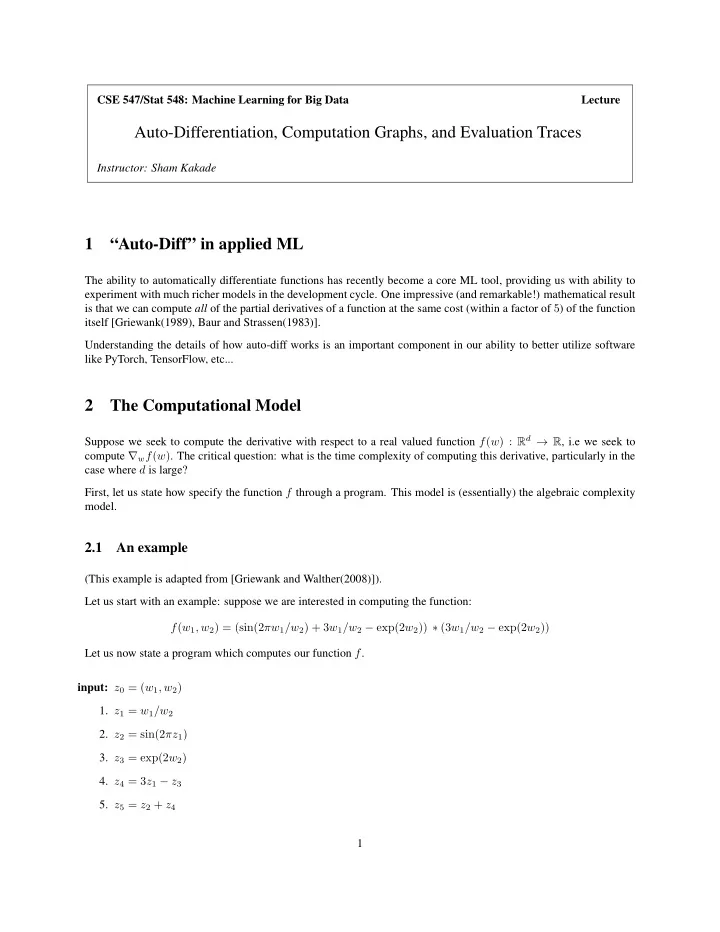
  1. CSE 547/Stat 548: Machine Learning for Big Data Lecture Auto-Differentiation, Computation Graphs, and Evaluation Traces Instructor: Sham Kakade 1 “Auto-Diff” in applied ML The ability to automatically differentiate functions has recently become a core ML tool, providing us with ability to experiment with much richer models in the development cycle. One impressive (and remarkable!) mathematical result is that we can compute all of the partial derivatives of a function at the same cost (within a factor of 5 ) of the function itself [Griewank(1989), Baur and Strassen(1983)]. Understanding the details of how auto-diff works is an important component in our ability to better utilize software like PyTorch, TensorFlow, etc... 2 The Computational Model Suppose we seek to compute the derivative with respect to a real valued function f ( w ) : R d → R , i.e we seek to compute ∇ w f ( w ) . The critical question: what is the time complexity of computing this derivative, particularly in the case where d is large? First, let us state how specify the function f through a program. This model is (essentially) the algebraic complexity model. 2.1 An example (This example is adapted from [Griewank and Walther(2008)]). Let us start with an example: suppose we are interested in computing the function: f ( w 1 , w 2 ) = (sin(2 πw 1 /w 2 ) + 3 w 1 /w 2 − exp(2 w 2 )) ∗ (3 w 1 /w 2 − exp(2 w 2 )) Let us now state a program which computes our function f . input: z 0 = ( w 1 , w 2 ) 1. z 1 = w 1 /w 2 2. z 2 = sin(2 πz 1 ) 3. z 3 = exp(2 w 2 ) 4. z 4 = 3 z 1 − z 3 5. z 5 = z 2 + z 4 1

  2. 6. z 6 = z 4 z 5 return: z 6 Our “program” is sometimes referred to as an evaluation trace , when written in this manner. The computation graph is the flow of operations. For example, here z 1 points to z 2 and z 4 ; z 2 points to z 5 ; z 4 points to z 5 and z 6 ; etc. We say that z 2 and z 4 and children of z 1 ; z 5 is a child of z 2 ; etc. 2.2 The computation graph and evaluation traces Now let us specify the model more abstractly. Suppose we have access to a set of differentiable real value functions h ∈ H . The computational model is one where we use our functions in H to create intermediate variables. Specifically, our evaluation trace will be of the form: input: z 0 = w . We actually have d (scalar) input nodes where [ z 0 ] 1 = w 1 , [ z 0 ] 2 = w 2 , . . . [ z 0 ] 3 = w d . 1. z 1 = h 1 ( a fixed subset of the variables in w ) . . . t. z t = h t ( a fixed a subset of the variables in z 1: t − 1 , w ) . . . T. z T = h T ( a fixed a subset of the variables in z 1: T − 1 , w ) return: z T . Let us say every h ∈ H is one of the following: 1. an affine transformation of the inputs (e.g. step 4 in our example) 5 z − 1 2. a product of variables, to some power (e.g. step 1, step 6 in our example. we could also have z 8 = z 4 1 ∗ z 7 6 ). 3. h could lie in some fixed set of one dimensional differentiable functions. Examples include sin( · ) , cos( · ) , exp( · ) , log( · ) , etc. Implicitly, we are assuming that we can “easily” compute the derivatives for each of these one dimensional functions h (we specify this precisely later on). For example, we could have z 8 = sin(2 z 3 ) . We do not allow z 8 = sin(2 z 3 + 7 z 5 + z 6 ) ; for the latter, we would have to create another intermediate variable for 2 z 3 + 7 z 5 + z 6 . This restriction is to make our computations as efficient as possible. Remark: We don’t really need the functions of type 3 . In a very real sense, all our transcendental functions like sin( · ) , cos( · ) , exp( · ) , log( · ) , etc. are all implemented (in code) through using functions of type 1 and 2 , e.g. when you call the sin( · ) function, it is computed through a polynomial. Relation to Backprop and a Neural Net: In the special case of neural nets, note that our computation graph should not be thought of as being the same as the neural net graph. With regards to the computation graph, the input nodes are w . In a neural net, we often think of the input as x . Note that for neural nets which are not simple MLPS (say you have skip connections or one which is more generally a DAG), then there are multiple ways ot execute the computation, giving rise to different computational graphs, and this order is relevant in how we execute the reverse mode. 2

  3. 3 The Reverse Mode of Automatic Differentiation The subtle point in understanding auto-diff is understanding the chain rule due to that all z t are dependent variables on z 1: t − 1 and w . It is helpful to think of z T as a function of both a single grandparent z t along with w as follows (slightly, abusing notation): z T = z T ( w, z t ) where think of z t as a free variable. In particular, this means we think of z T as being computed by following the evaluation trace (our program) except that at node t it uses the value z t ; this node ignores its inputs and is “free” to use another value z t instead. In this sense, we think of z t as a free variable (not depending on w or on any of its parents). We will be interested in computing the derivatives (again, slightly abusing notation): dz T := dz T ( w, z t ) dz t dz t for all the variables z t . With this definition, the chain rule implies that: dz T dz T ∂z c � = (1) dz t dz c ∂z t c is a child of t where the sum is over all children of t . Here, a child is a node in the computation graph which z t directly points to. Now the algorithm can be defined as follows. 1. Compute f ( w ) and store in memory all the intermediate variables z 0: T . 2. Initialize: dz T = 1 dz T 3. Proceeding recursively, starting at t = T − 1 and going to t = 0 dz T dz T ∂z c � = dz t dz c ∂z t c is a child of t dz 0 = d f 4. return dz T dw dz 0 = d f Note that dz T dw by the definition of z T and z 0 . 4 Time complexity The following theorem has been proven independently [Griewank(1989), Baur and Strassen(1983)]. In computer sci- ence theory, it is often referred to as the Baur-Strassen theorem. Theorem 4.1. ([Griewank(1989), Baur and Strassen(1983)]) Assume that every h ( · ) is specified as in our compu- tational model (with the aforementioned restrictions). Furthermore , for h ( · ) of type 3, let us assume that we can compute the derivative of h ′ ( z ) in time that is within a factor of 5 of computing h ( z ) itself. Using a given evaluation trace, let T be the time it takes to compute f ( w ) at some input w , then the reverse mode computes both f ( w ) and d f dw in time 5 T . In other words, we compute all d partial derivatives of f in essentially the same time as computing f itself. 3

  4. Proof. First, let us show the algorithm is correct. The equation to compute dz T dz t follows from the chain rule. Further- more, based on the order of operations, at (backward) iteration t, we have already computed dz T dz c for all children c of t . Now let us observe that we can compute ∂z c ∂z t using the variables stored in memory. To see this, consider our three cases (and let us observe the computational cost as well): 1. If h is affine, the derivative is simply the coefficient of z t . 2. If h is a product of terms (possibly with divisions), then ∂z c ∂z t = z c ( α/z t ) , where alpha is the power of z t . For 4 we have that ∂z 5 example, for z 5 = z 2 z 2 ∂z 4 = z 5 ∗ (2 /z 4 ) . 3. If z c = h ( z t ) (so it is a one dim function of just one variable), then ∂z c ∂z t = h ′ ( z t ) . Hence, the algorithm is correct, and the derivates are computable using what we have stored in memory. Now let us verify the claimed time complexity. The compute time T for f ( w ) is simply the sum of times required to compute z 1 to z T . We will relate this time to the time complexity of the reverse mode. In the reverse mode, note that since ∂z c ∂z t is used precisely once: it is computed when we hit node t . Now let us show that the compute time of z c and the compute time for computing all the derivatives { ∂z c ∂z t : t which are parents of c } are of the same order. If z c is an affine function of its parents — suppose there are M parents — then z c takes time O ( M ) time to compute and computing all the partial derivatives also takes O ( M ) in total: each ∂z c ∂z t is O (1) (since the derivative is just a constant) there are M such derivatives. A similar argument can be made for case 2 . For case 3 , computing ∂z c ∂z t (for the only parent t ) is the same order as computing z c by assumption. Hence, we have show that computing z c and computing all the derivatives { ∂z c ∂z t : t which are parents of c } are of the same order. This accounts for all the computation required to compute all the ∂z c ∂z t ’s. It is now straightforward to see that the remaining computation of all the dz T dz t ’s using these partial derivatives, is also of order T , since each ∂z c ∂z t occurs just once in some sum. The factor of 5 is simply more careful book-keeping of the costs. References [Griewank(1989)] Andreas Griewank. On automatic differentiation. In IN MATHEMATICAL PROGRAMMING: RECENT DEVELOPMENTS AND APPLICATIONS , pages 83–108. Kluwer Academic Publishers, 1989. [Baur and Strassen(1983)] Walter Baur and Volker Strassen. The complexity of partial derivatives. Theoretical Com- puter Science , 22:317–330, 1983. [Griewank and Walther(2008)] Andreas Griewank and Andrea Walther. Evaluating Derivatives: Principles and Tech- niques of Algorithmic Differentiation . Society for Industrial and Applied Mathematics, Philadelphia, PA, USA, second edition, 2008. 4
Download Presentation
Download Policy: The content available on the website is offered to you 'AS IS' for your personal information and use only. It cannot be commercialized, licensed, or distributed on other websites without prior consent from the author. To download a presentation, simply click this link. If you encounter any difficulties during the download process, it's possible that the publisher has removed the file from their server.

Recommend


More recommend