
SLIDE 1
www.oerc.ox.ac.uk
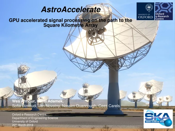
AstroAccelerate
GPU accelerated signal processing on the path to the Square Kilometre Array
Wes Armour, Karel Adamek, Sofia Dimoudi, Jan Novotny, Nassim Ouannough, Cees Carels
Oxford e-Research Centre, Department of Engineering Science University of Oxford 20th March 2019