Aperitif: Relational semantics of loops Automatic program - - PowerPoint PPT Presentation

— 1 —

« Automatic program verification by Lagrangian relaxation and semidefinite programming »

Patrick Cousot École normale supérieure 45 rue d’Ulm 75230 Paris cedex 05, France

Patrick.Cousot@ens.fr www.di.ens.fr/~cousot

Semantics lunch — Cambridge, UK — Oct. 18th, 2004

Aperitif: Relational semantics of loops

§

• x

x

§

— 3 —

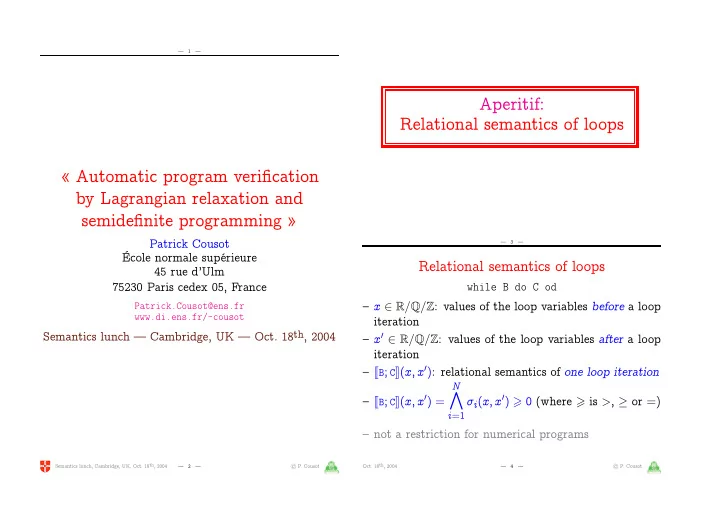
Relational semantics of loops

while B do C od – x 2 R=Q=Z: values of the loop variables before a loop iteration – x0 2 R=Q=Z: values of the loop variables after a loop iteration – B; C(x; x0): relational semantics of one loop iteration – B; C(x; x0) =

N

V

i=1

ffi(x; x0) > 0 (where > is >, – or =) – not a restriction for numerical programs

ľ P. Cousot

• Oct. 18th, 2004

Semantics lunch, Cambridge, UK, Oct. 18th, 2004 — 2 — — 4 — ľ P. Cousot

Example of quadratic form program (factorial)

[x x0]A[x x0]> + 2[x x0] q + r > 0

n := 0; f := 1; while (f <= N) do n := n + 1; f := n * f

• d
• 1.f +1.N >= 0

+1.n >= 0 +1.f -1 >= 0

• 1.n +1.n’ -1 = 0

+1.N -1.N’ = 0

• 1.f.n’ +1.f’ = 0

[nfNn0f0N0] 2 6 6 6 6 6 6 6 4 0 0 0 0 0 0 0 0 0 `1

2 0 0

0 0 0 0 0 0 0 `1

2 0 0 0 0

0 0 0 0 0 0 0 0 0 0 0 0 3 7 7 7 7 7 7 7 5 2 6 6 6 6 6 6 4 n f N n0 f0 N0 3 7 7 7 7 7 7 5 +2[nfNn0f0N0] 2 6 6 6 6 6 6 4

1 2

3 7 7 7 7 7 7 5 +0 = 0

— 5 —

Appetiser: Floyd/Hoare/Naur correctness proof method

Invariance proof

Given a loop precondition P, find an unkown loop in- variant I such that: – The invariant is initial: 8 x : P(x) ) I(x) – The invariant is inductive: 8 x; x0 : I(x) ^ B; C(x; x0) ) I(x0)

— 7 —

Invariance proof for numerical programs

Given a loop precondition P(x) > 0, find an unkown loop invariant I(x) > 0 such that: – The invariant is initial: 8 x : P(x) > 0 ) I(x) > 0 – The invariant is inductive: 8 x; x0 : B @I(x) > 0 ^

N

^

i=1

ffi(x; x0) > 0 1 C A ) I(x0) > 0

ľ P. Cousot

• Oct. 18th, 2004

Semantics lunch, Cambridge, UK, Oct. 18th, 2004 — 6 — — 8 — ľ P. Cousot

Termination proof

Given a loop invariant I, find an R=Q=Z-valued unkown rank function r such that: – The rank is nonnegative: 8 x : I(x) ) r(x) – 0 – The rank is strictly decreasing: 8 x; x0 : I(x) ^ B; C(x; x0) ) r(x0) » r(x) ` ” ” = 1 for Z, ” > 0 for R=Q to avoid Zeno 1

2, 1 4, 1

• 8. . .

— 9 —

Wine service: Iterated forward/backward static analysis for conditional termination

Conditional termination

– In general a loop does not terminate for all initial val- ues of the variables – In that case we can find no rank function! – We must automatically determine a necessary loop precondition – We use a iterated forward/backward static analysis . . . with an auxiliary counter counting the number of re- maining iterations down to zero

— 11 —

Arithmetic mean example, polyhedral abstraction without auxiliary counter)

{x>=y} while (x <> y) do {x>=y+2} x := x - 1; {x>=y+1} y := y + 1 {x>=y}

• d

{x=y}

ľ P. Cousot

• Oct. 18th, 2004

Semantics lunch, Cambridge, UK, Oct. 18th, 2004 — 10 — — 12 — ľ P. Cousot

Arithmetic mean example, polyhedral abstraction with auxiliary counter

{x=y+2k,x>=y} while (x <> y) do {x=y+2k,x>=y+2} k := k - 1; {x=y+2k+2,x>=y+2} x := x - 1; {x=y+2k+1,x>=y+1} y := y + 1 {x=y+2k,x>=y}

• d

{x=y,k=0} assume (k = 0) {x=y,k=0}

— 13 —

Entrée: Abstraction to parametric constraints

Parametric constraints

– Fix the form of the unkown (I(x) > 0/r(x) > 0) using parameters a in the form Q(a; x) > 0 – This is an abstraction – Examples:

• r(x; y) = a:x + b:y + c
• I(x; x0) = a:x2 + b:x:x0 + c:x02 + d:x + e:x0 + f

— 15 —

Solving the constraints

– The invariance [termination] problems have the form: 9 a : 8 x; x0 : B @[Q(a; x) > 0 ^ ]

n

^

k=1

Ck(x; x0) > 0 1 C A ) Q0(a; x; x0) > 0 – Find an algorithm to effectively compute a!

ľ P. Cousot

• Oct. 18th, 2004

Semantics lunch, Cambridge, UK, Oct. 18th, 2004 — 14 — — 16 — ľ P. Cousot

Problems

In order to compute a: – How to handle V ? – How to get rid of the implication ) ? ! Lagrangian relaxation – How to get rid of the universal quantification 8 ? – How to handle ^ ? ! quantifier elimination (does not scale up) ! mathematical programming

— 17 —

Algorithmically interesting cases

– linear inequalities ! linear programming 1 – linear matrix inequalities (LMI)/quadratic forms – bilinear matrix inequalities (BMI) ! semidefinite programming – semialgebraic sets ! polynomial quantifier elimination, or ! relaxation with semidefinite programming

1 Already explored for invariants by Sankaranarayanan, Spima, Manna (CAV’03, SAS’04, heuristic solver) and for termination by Podelski & Rybalchenko (VMCAI’03, Lagrange coefficients eliminated by hand to reduce to linear programming so no disjunctions, no tests, etc).

First main course: Lagrangian relaxation for implication elimination

— 19 —

Example of linear Lagrangian relaxation

A ) B (assuming A 6= ;) ( (soundness) ) (completeness) border of A parallel to border of B

ľ P. Cousot

• Oct. 18th, 2004

Semantics lunch, Cambridge, UK, Oct. 18th, 2004 — 18 — — 20 — ľ P. Cousot

Lagrangian relaxation, formally

Let V be a finite dimensional linear vector space, N > 0 and 8k 2 [1; N] : ffk 2 V 7! R. 8x 2 V : @

N

^

k=1

ffk(x) – 0 1 A ) (ff0(x) – 0) ( soundness (Lagrange) ) completeness (lossless) 6) incompleteness (lossy) 9– 2 [1; N] 7! R˜ : 8x 2 V : ff0(x) `

N

X

k=1

–kffk(x) – 0 relaxation = approximation, –i = Lagrange coefficients

— 21 —

Lagrangian relaxation, completeness cases

– Linear case (affine Farkas’ lemma) – Linear case with at most 2 quadratic constraints (Yakubovich’s S-procedure)

Lagrangian relaxation of the constraints

9 a : 8 x; x0 : [Q(a; x) > 0 ^ ]

n

^

k=1

Ck(x; x0) > 0 ) Q0(a; x; x0) > 0 ( (is relaxed into) 9 a : [9– > 0] : 9–k > 0 : 8 x; x0 : Q0(a " linear in a ; x; x0)[ ` – " bilinear in a & – :Q(a; x)] `

n

X

k=1

–k " linear in the –k :Ck(x; x0) > 0

— 23 —

Second main course: Mathematical programming for quantifier elimination

ľ P. Cousot

• Oct. 18th, 2004

Semantics lunch, Cambridge, UK, Oct. 18th, 2004 — 22 — — 24 — ľ P. Cousot

Mathematical programming

9x 2 Rn:

N

^

i=1

gi(x) > 0 [Minimizing f(x)] feasibility problem : find a solution to the constraints

• ptimization problem : find a solution, minimizing f(x)

— 25 —

Semidefinite programming, once again

9x 2 Rn: M(x) < 0 [Minimizing cx] Where the linear matrix inequality is M(x) = M0 +

n

X

k=1

xkMk with symetric matrices (Mk = Mk> and the positive semidefiniteness is M(x) < 0 = 8X 2 RN : X>M(x)X – 0

Semidefinite programming, once again

Feasibility is: 9x 2 Rn: 8X 2 RN : X> @M0 +

n

X

k=1

xkMk 1 A X – 0

• f the form of the (linear) formulæ we are interested in

for programs with linear matricial semantics.

— 27 —

Interior point method for semidefinite programming

– Nesterov & Nemirovskii 1988, polynomial in worst case and good in practice (thousands of variables)

x x

– Various path strategies e.g. “stay in the middle”

ľ P. Cousot

• Oct. 18th, 2004

Semantics lunch, Cambridge, UK, Oct. 18th, 2004 — 26 — — 28 — ľ P. Cousot

Semidefinite programming solvers

Numerous solvers available under Mathlab

ő, a.o.:

– lmilab: P. Gahinet, A. Nemirovskii, A.J. Laub, M. Chilali – Sdplr: S. Burer, R. Monteiro, C. Choi – Sdpt3: R. Tütüncü, K. Toh, M. Todd – SeDuMi: J. Sturm – bnb: J. Löfberg (integer semidefinite programming) Common interfaces to these solvers, a.o.: – Yalmip: J. Löfberg Sometime need some help (feasibility radius, shift,. . . )

— 29 —

Recent generalization to bilinear matrix inequalities

– penbmi: M. Kočvara, M. Stingl Feasibility is: 9x 2 Rn : 8X 2 RN : X> @M0 +

n

X

j=1

xjMj +

n

X

k=1 n

X

‘=1

xkx‘M0

k‘

1 A X – 0

• f the form of the (bilinear) formulæ we are interested

in!

Skipping the cheese . . .

— 31 —

Not enough time for . . .

– Disjunctions in the loop test? – Conditionals in the loop body? – Nested loops? – Concurrency? – Fair parallelism? – Semi-algebraic/polynomial programs? – Data structures?

ľ P. Cousot

• Oct. 18th, 2004

Semantics lunch, Cambridge, UK, Oct. 18th, 2004 — 30 — — 32 — ľ P. Cousot

Desert Invariance and Termination Examples

— 33 —

Termination of a linear program

{y >= 1} ` termination precondition de- termined by iterated for- ward/backward polyhedral analysis while (x >= 1) do x := x - y

• d

lmilab: r(x,y) = +2.178955e+12.x +1.453116e+12.y -1.451513e+12 lmilab (with feasibility radius of 1.0e4): r(x,y) = +4.074723e+03.x +2.786715e+03.y +1.549410e+03 sedumi: r(x,y) = +2.271450e+03.x +1.810903e+03.y -3.623997e+03 bnb (integer semidefinite programming) 2: r(x,y) = +2.x+2.y-3

2 still in infancy!

Termination of the arithmetic mean

{x=y+2k,x>=y} ` termination precondition determined by iterated forward/backward poly- hedral analysis while (x <> y) do k := k - 1; x := x - 1; y := y + 1

• d

{assert (k = 0)} lmilab:

r(x,y,k) = +1.382113e+03.x -1.382113e+03.y +4.978695e+03.k +2.711732e+03

— 35 —

Termination of the Euclidean division

1: {y>=1} ` termination precondition determined by iterated forward/backward polyhe- dral analysis bnb: r(y,q,r) = -2.y +2.q +4.r Floyd’s proposal r(x; y; q; r) = x ` q is more intuitive but requires to discover the nonlinear loop invariant x = r +qy. q := 0; 2: {q=0,y>=1} r := x; 3: {x=r,q=0,y>=1} while (y <= r) do 4: {y<=r,q>=0} r := - y + r; 5: {r>=0,q>=0} q := q + 1 6: {r>=0,q>=1}

• d

7: {q>=0,y>=r+1}

ľ P. Cousot

• Oct. 18th, 2004

Semantics lunch, Cambridge, UK, Oct. 18th, 2004 — 34 — — 36 — ľ P. Cousot

Termination of a quadratic program: factorial

{true} ` termination precondition determined by iterated for- ward/backward polyhedral analysis n := 0; f := 1; while (f <= N) do n := n + 1; f := n * f

• d

sedumi (with feasibility radius of 1.0e+3):

r(n,f,N) = -9.993462e-01.n +1.617225e-04.f +2.688476e+02.N +8.745232e+02

— 37 —

Loop body with tests

while (x < y) do if (i >= 0) then x := x+i+1 else y := y+i fi

• d

lmilab:

r(i,x,y) = -2.252791e-09.i -4.355697e+07.x +4.355697e+07.y +5.502903e+08

Quadratic termination of linear loop

{n>=0} ` termination

precondition determined by iterated for- ward/backward polyhedral analysis

i := n; j := n; while (i <> 0) do if (j > 0) then j := j - 1 else j := n; i := i - 1 fi

• d

— 39 —

sdplr (with feasibility radius of 1.0e+3):

r(n,i,j) = +7.024176e-04.n^2 +4.394909e-05.n.i ...

• 2.809222e-03.n.j +1.533829e-02.n ...

+1.569773e-03.i^2 +7.077127e-05.i.j ... +3.093629e+01.i -7.021870e-04.j^2 ... +9.940151e-01.j +4.237694e+00 Successive values

• f

r(n; i; j) for n = 10 on loop entry

5 10 2 4 6 8 10 50 100 150 200 250 300 350

j Ranking function i r(10,i,j)

ľ P. Cousot

• Oct. 18th, 2004

Semantics lunch, Cambridge, UK, Oct. 18th, 2004 — 38 — — 40 — ľ P. Cousot

Termination of a concurrent program

[| 1: while [x+2 < y] do 2: [x := x + 1]

• d

3: || 1: while [x+2 < y] do 2: [y := y - 1]

• d

3: |]

interleaving

` !

while (x+2 < y) do if ?=0 then x := x + 1 else if ?=0 then y := y - 1 else x := x + 1; y := y - 1 fi fi

• d

penbmi: r(x,y) = 2.537395e+00.x+-2.537395e+00.y+

• 2.046610e-01

— 41 —

Termination of a fair parallel program

[[ while [(x>0)|(y>0) do x := x - 1] od || while [(x>0)|(y>0) do y := y - 1] od ]]

interleaving + scheduler

` !

{m>=1} termination precondition determined by iterated

forward/backward polyhedral analysis

t := ?; assume (0 <= t & t <= 1); s := ?; assume ((1 <= s) & (s <= m)); while ((x > 0) | (y > 0)) do if (t = 1) then x := x - 1 else y := y - 1 fi; s := s - 1; if (s = 0) then if (t = 1) then t := 0 else t := 1 fi; s := ?; assume ((1 <= s) & (s <= m)) else skip fi

• d;;

penbmi: r(x,y,m,s,t) = +1.000468e+00.x +1.000611e+00.y +2.855769e-02.m -3.929197e-07.s +6.588027e-06.t +9.998392e+03

Semidefinite programming relaxation for polynomial programs

eps = 1.0e-9; while (0 <= a) & (a <= 1 - eps) & (eps <= x) & (x <= 1) do x := a*x*(1-x)

• d

Write the verification conditions in polynomial form, use SOStool to relax in semidefinite programming form. SOStool+SeDuMi: r(x) = 1.222356e-13.x + 1.406392e+00

— 43 —

When constraint resolution fails. . .

Infeasibility of the constraints does not mean “non ter- mination” but simply failure: – There can be a rank function of a different form (e.g. quadratic while looking for a linear one), – The solver may have failed (e.g. add a shift).

ľ P. Cousot

• Oct. 18th, 2004

Semantics lunch, Cambridge, UK, Oct. 18th, 2004 — 42 — — 44 — ľ P. Cousot

Coffee: Conclusion

— 45 —

Numerical errors

– LMI solvers do numerical computations with rounding errors, shifts, etc – rank function is subject to numerical errors – the hard point is to discover a candidate for the rank function – much less difficult, when it is known, to re-check for satisfaction (e.g. by static analysis)

Invariance for Euclidian division

assume (y > 0); q := 0; r := x; while (y <= r) do r := - y + r; q := q + 1

• d

yalmip bmi: 1.337645e-04*x+2.484973e-04*q*y+1.588933e-03*r >= 0 which is not false!

— 47 —

Digestif: Questions

ľ P. Cousot

• Oct. 18th, 2004

Semantics lunch, Cambridge, UK, Oct. 18th, 2004 — 46 — — 48 — ľ P. Cousot

Seminal work

– LMI case, Lyapunov 1890, “an invariant set of a dif- ferential equation is sta- ble in the sense that it at- tracts all solutions if one can find a function that is bounded from below and decreases along all solu- tions outside the invariant set”.

— 49 —

THE END I hope you had a good and relaxed semantics lunch

ľ P. Cousot

• Oct. 18th, 2004

Semantics lunch, Cambridge, UK, Oct. 18th, 2004 — 50 — ľ P. Cousot