[Andrieu, Doucet & Holenstein, 2010] Introduce algorithms that - - PowerPoint PPT Presentation

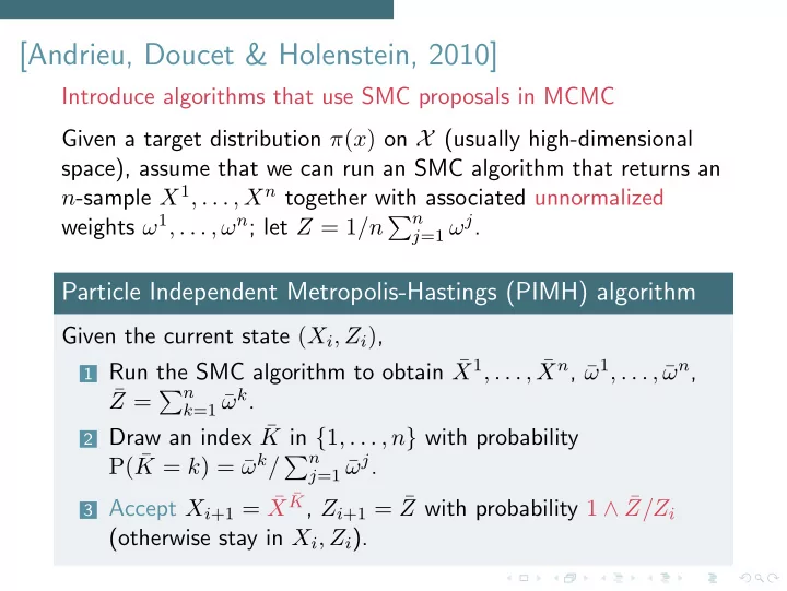
[Andrieu, Doucet & Holenstein, 2010]

Introduce algorithms that use SMC proposals in MCMC Given a target distribution π(x) on X (usually high-dimensional space), assume that we can run an SMC algorithm that returns an n-sample X1, . . . , Xn together with associated unnormalized weights ω1, . . . , ωn; let Z = 1/n n

j=1 ωj.

Particle Independent Metropolis-Hastings (PIMH) algorithm

Given the current state (Xi, Zi),

1 Run the SMC algorithm to obtain ¯

X1, . . . , ¯ Xn, ¯ ω1, . . . , ¯ ωn, ¯ Z = n

k=1 ¯

ωk.

2 Draw an index ¯

K in {1, . . . , n} with probability P( ¯ K = k) = ¯ ωk/ n

j=1 ¯

ωj.

3 Accept Xi+1 = ¯

X ¯

K, Zi+1 = ¯

Z with probability 1 ∧ ¯ Z/Zi (otherwise stay in Xi, Zi).

Proof [Assuming that ( ¯

Xj, ¯ ωj)j=1,...,n is produced by direct importance sampling with instrumental pdf q (i.e. no resampling)]

1 The important idea is that the state of the chain is in fact

(X1, . . . , Xn, K) and that the targeted auxiliary distribution has pdf πaux(x1, . . . , xn, k) = 1 nπ(xk)

• j=k

q(xj)

2 Check that indeed XK has marginal distribution π under πaux 3 The proposal distribution is independent of the current state

and is given by qaux(¯ x1, . . . , ¯ xn, ¯ k) = π(¯ x¯

k)/q(¯

x¯

k)

• l π(¯

xl)/q(¯ xl)

• j

q(¯ xj)

4 The Metropolis-Hastings acceptance ratio is given by

πaux(¯ x1, . . . , ¯ xn, ¯ k) πaux(x1, . . . , xN, k) qaux(x1, . . . , xn, k) qaux(¯ x1, . . . , ¯ xN, ¯ k) = ¯ z z as πaux(¯ x1, . . . , ¯ xn, ¯ k) qaux(¯ x1, . . . , ¯ xn, ¯ k) =

1 nπ(¯

x¯

k) j=¯ k q(¯

xj)

π(¯ x¯

k)/q(¯

x¯

k)

P

l π(¯

xl)/q(¯ xl)

• j q(¯

xj) = 1 n

• l

π(¯ xl)/q(¯ xl) = ¯ z

5 Keeping the whole state (X1, . . . , Xn, K) is not required and

• ne only needs to keep track of XK and Z

The method can defeat the curse of dimensionality (at a certain price...)

10 10

1

10

2

10

3

10

1

10

2

10

3

10

4

Dimension T ACCEPTANCE RATE Number N of Particles

0.1 0.2 0.3 0.4 0.5 0.6 0.7 0.8 0.9 1

Figure: PIMH acceptance rate as a function of the dimension T of the target and the number N of particles.

The target pdf is πT (x1, . . . , xT ) = QT

t=1 π(xt), where π is the normal pdf truncated to the range [−4, 4];

the SMC proposal “kernel” q is an independent proposal, uniformly distributed in the range [−4, 4]. To assess the difficulty of the simulation task, note that for direct self-normalized importance sampling targeting πT the Effective Sample Size (ESS) statistic, normalized by N, tends to 2.26−T (2.26 = R 4

−4 8π2(x)dx) as N

increases, which is about 10−6 for T = 17.