an introduction to computational psycholinguistics
play

An introduction to computational psycholinguistics: Modeling human - PDF document

An introduction to computational psycholinguistics: Modeling human sentence processing Shravan Vasishth University of Potsdam, Germany http://www.ling.uni-potsdam.de/ vasishth vasishth@acm.org September 2005, Bochum Neural structure 1 A
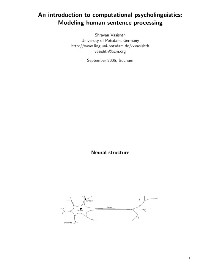

  1. An introduction to computational psycholinguistics: Modeling human sentence processing Shravan Vasishth University of Potsdam, Germany http://www.ling.uni-potsdam.de/ ∼ vasishth vasishth@acm.org September 2005, Bochum Neural structure 1

  2. A model of the neuron 2 Activation functions for translating net input to activation 3

  3. A model of layered neural connections 4 Five assumptions • Neurons integrate information • Neurons pass information about the level of their input. • Brain structure is layered. • The influence of one neuron on another depends on the strength of the connection between them. • Learning is achieved by changing the strengths of the connections between neurons. 5

  4. The computations Net input to unit i from units j = 1 . . . n each with activation a j , and with weight of connection from j to i being w ij : n X Netinput i = a j w ij (1) j =  Activation a i of unit i, f an activation function from inputs to activation values: a i = f ( netinput i ) (2) 6 Learning by weight change n X Netinput i = a j w ij (3) j =  a i = f ( netinput i ) (4) • Notice that the activity of i , a i , is a function of the weights w ij and the activations a j . So changing w ij will change a i . • In order for this simple network to do something useful, for a given set of input activations a j , it should output some particular value for a i . Example: computing the logical AND function. 7

  5. The AND network: the single-layered perceptron Assume a threshold activation function: if netinput i is greater than 0 , output a 1 . Bias is − 1 . 5 . Netinput  =0 × 1 + 0 × 1 − 1 . 5 = − 1 . 5 (5) Netinput  =0 × 1 + 1 × 1 − 1 . 5 = − 0 . 5 (6) Netinput  =1 × 1 + 0 × 1 − 1 . 5 = − 0 . 5 (7) Netinput  =1 × 1 + 1 × 1 − 1 . 5 = +0 . 5 (8) 8 How do we decide what the weights are? Let the w j = . . Now the same network fails to compute AND. Netinput  =0 × 0 . 5 + 0 × 0 . 5 − 1 . 5 = − 1 . 5 (9) Netinput  =0 × 0 . 5 + 1 × 0 . 5 − 1 . 5 = − 1 (10) Netinput  =1 × 0 . 5 + 0 × 0 . 5 − 1 . 5 = − 1 (11) Netinput  =1 × 0 . 5 + 1 × 0 . 5 − 1 . 5 = − 0 . 5 (12) 9

  6. The Delta rule for changing weights to get the desired output We can repeatedly cycle through the simple network and adjust the weights so that we achieved the desired a i . Here’s a rule for doing this: ∆ w ij = [ a i (desired) − a i (obtained) ] a j ǫ (13) ǫ : learning rate parameter (determines how large the change will be on each learning trial) This is, in effect, a process of learning. 10 How the delta rule fixes the weights in the AND network ∆ w ij = [ a i (desired) − a i (obtained) ] a j ǫ (14) Let a i (desired) =  ; ǫ = 0 . 5 . Consider now the activations we get: Netinput  =0 × 0 . 5 + 0 × 0 . 5 − 1 . 5 = − 1 . 5 (15) Netinput  =0 × 0 . 5 + 1 × 0 . 5 − 1 . 5 = − 1 (16) Netinput  =1 × 0 . 5 + 0 × 0 . 5 − 1 . 5 = − 1 (17) Netinput  =1 × 0 . 5 + 1 × 0 . 5 − 1 . 5 = − 0 . 5 ⇐ (18) We don’t need to mess with the first three since we already have a desired value (less than zero). Look at the last one. Say desired a  =  . 11

  7. ∆ w i = [ a i (desired) − a i (obtained) ] a  ǫ (19) = [1 − ( − 0 . 5)] × 1 × 0 . 5 (20) = . 75 (21) We just performed what’s called a a training sweep . Sweep : the presentation of a single input pattern causing activation to propagate through the network and the appropriate weight adjustments to be carried out. Epoch : One cycle of showing all the inputs in turn. Now if we recompute the netinput with the incremented weights, our network starts to behave as intended: Netinput  =1 × 1 . 25 + 1 × 1 . 25 − 1 . 5 = 1 (22) 12 Rationale for the delta rule ∆ w ij = [ a i (desired) − a i (obtained) ] a j ǫ (23) • If obtained activity is too low, then [ a i (desired) − a i (obtained) ] >  . This increases the weight. • If obtained activity is too high, then [ a i (desired) − a i (obtained) ] <  . This decreases the weight. • For any input unit j , the greater its activation a j the greater its influence on the weight change. The delta rule concentrates the weight change to units with high activity because these are the most influential in determining the (incorrect) output. There are other rules one can use. This is just an example of one of them. 13

  8. Let’s do some simulation with tlearn DEMO: Steps • Create a network with 2 input and 1 one output node (plus a bias node with a fixed output) • Create a data file, and a teacher: the data file is the input and the teacher is the output you want the network to learn to produce. Input Output 0 0 0 1 0 0 0 1 0 1 1 1 • Creating the network 14 The AND network’s configuration NODES:#define the nodes nodes = 1 # number of units (excluding input units) inputs = 2 # number of input nodes outputs = 1 # number of output nodes output node is 1 #always start counting output nodes from 1 CONNECTIONS: groups = 0 # how many groups of connections must have same value? 1 from i1-i2 #connections 1 from 0 #bias node is always numbered 0, it outputs 1 SPECIAL: selected = 1 # units selected for printing out the output of weight_limit = 1.0 # causes initial weights to be +/-0.5 15

  9. Training the network • Set the training sweeps, learning rate (how fast weights change), the momentum (how similar is the weight change from one cycle to the next—helps avoid local maxima), random seed (for the initial random weights), training method (random or sequential), • We can compute the error in any one case: desired-actual. • How to evaluate (quantify) the performance of the network as a whole? Note that the network will give four different actual activations in response to the four input pairs. We need some notion of average error . • Suggestions? 16 Average error: Root mean square r P ( tk − ok )  j Root mean square error = k 17

  10. Exercise: Learning OR • Build a network that can recognize logical OR and then XOR. • Are these two networks also able to learn using the procedure we used for AND? Readings for tomorrow: Elman 1990, 1991, 1993. Just skim them. 18 How to make the network predict what will come next? Key issue: if we want the network to predict, we need to have a notion of time, of now and now+1. Any suggestions? 19

  11. Simple recurrent networks • Idea: Use recurrent connections to provide the network with a dynamic memory. • The hidden node activation at time step t − 1 will be fed right back to the hidden nodes at time t (the regular input nodes will also be providing input to the hidden nodes). Context nodes serve to tell the network what came earlier in time. output, y(t) hidden, z(t) copy z input, x(t) hidden, z(t-1) 20 Let’s take up the demos Your printouts contain copies of Chapters 8 and 12 of Exercises in rethinking innateness , Plunkett and Elman. 21

  12. Elman 1990 22 Christiansen and Chater on recursion • Chomsky showed that natural language grammars exhibit recursion, and that this rules out finite state machines as models of language • According to Chomsky, this entails that language is innate: the child’s language exposure involves so few recursive structures that it could not possible learn recursion from experience • C(hristiansen+Chater): if connectionist models can reflect the limits on our ability to process recursion, they constitute a performance model • C notes a broader issue: Symbolic rules apply without limit (infinitely), but in the real-life we observe (though experiments) limits on processing ability. The reason for this boundedness of processing falls out of the hardware’s (wetware’s) architecture • C proceeds to demonstrate that human constraints on processing recursion fall out from the architecture of simple recurrent networks 23

  13. Three kinds of recursion (acc. to Chomsky) 1. Counting recursion: a n b n 2. Cross-serial embeddings: a n b m c n d m 3. Center embeddings: a n b m c m d n 4. (Baseline: right-branching) 24 Benchmark: n-gram models • In order to compare their results with an alternative frequency-based method of computing predictability, they looked at the predictions made by 2- and 3-gram models. • Diplomarbeit topic : try to find a better probabilistic parsing measure of predicting the next word, compared to the SRN baseline. In John Hale’s work we will see an example (though the goal of that work is different from the present discussion). 25

  14. Three distinct languages All languages contain only nouns (Ns) and verbs (Vs), both singular and plural: • L1: a N a N b V b V (ignores agreement) • L2: a N b V b V a N (respects agreement) • L3: a N b N a V b V (respects agreement) • Each language also had right-branchings: a N a V b N b V (respects agreement) 26 Method 27

Download Presentation
Download Policy: The content available on the website is offered to you 'AS IS' for your personal information and use only. It cannot be commercialized, licensed, or distributed on other websites without prior consent from the author. To download a presentation, simply click this link. If you encounter any difficulties during the download process, it's possible that the publisher has removed the file from their server.

Recommend


More recommend