{ a) policy evaluation (treatment effects ) Old b) attribution - PDF document

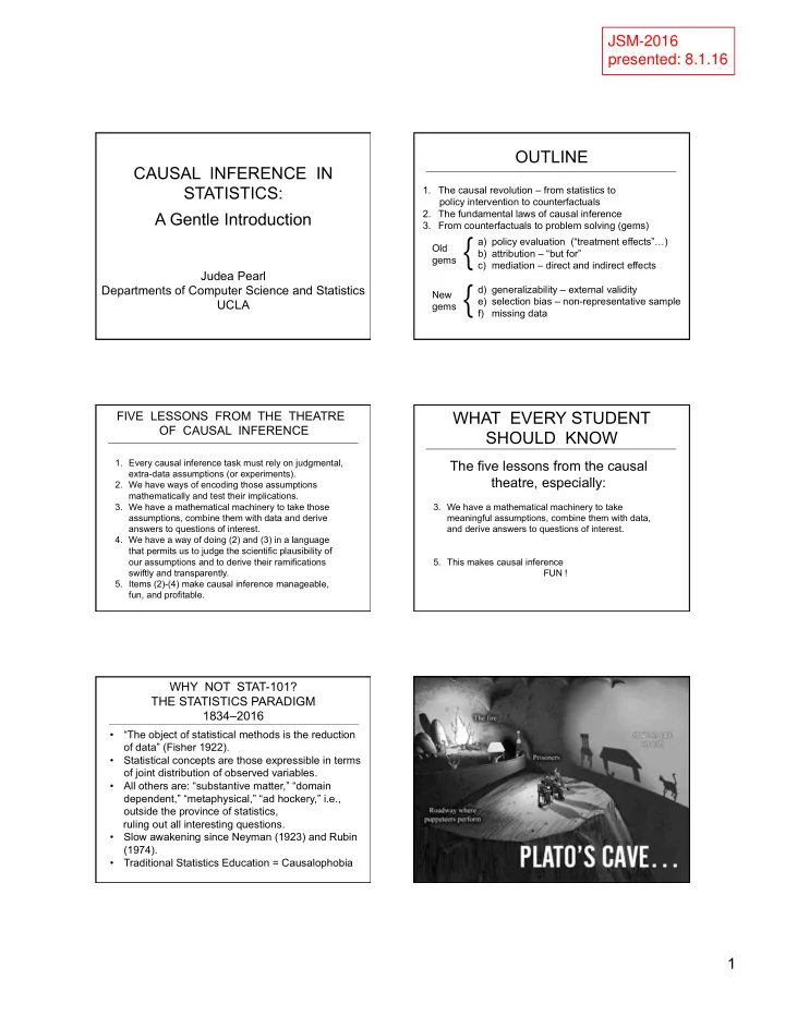
JSM-2016 presented: 8.1.16 OUTLINE CAUSAL INFERENCE IN STATISTICS: 1. The causal revolution – from statistics to policy intervention to counterfactuals 2. The fundamental laws of causal inference A Gentle Introduction 3. From counterfactuals to problem solving (gems) { a) policy evaluation (“treatment effects” … ) Old b) attribution – “but for” gems c) mediation – direct and indirect effects Judea Pearl gems { Departments of Computer Science and Statistics d) generalizability – external validity New e) selection bias – non-representative sample UCLA f) missing data WHAT EVERY STUDENT FIVE LESSONS FROM THE THEATRE OF CAUSAL INFERENCE SHOULD KNOW 1. Every causal inference task must rely on judgmental, The five lessons from the causal extra-data assumptions (or experiments). theatre, especially: 2. We have ways of encoding those assumptions mathematically and test their implications. 3. We have a mathematical machinery to take those 3. We have a mathematical machinery to take assumptions, combine them with data and derive meaningful assumptions, combine them with data, answers to questions of interest. and derive answers to questions of interest. 4. We have a way of doing (2) and (3) in a language that permits us to judge the scientific plausibility of our assumptions and to derive their ramifications 5. This makes causal inference swiftly and transparently. FUN ! 5. Items (2)-(4) make causal inference manageable, fun, and profitable. WHY NOT STAT-101? THE STATISTICS PARADIGM 1834–2016 • “The object of statistical methods is the reduction of data” (Fisher 1922). • Statistical concepts are those expressible in terms of joint distribution of observed variables. • All others are: “substantive matter,” “domain dependent,” “metaphysical,” “ad hockery,” i.e., outside the province of statistics, ruling out all interesting questions. • Slow awakening since Neyman (1923) and Rubin (1974). • Traditional Statistics Education = Causalophobia 1

TRADITIONAL STATISTICAL THE CAUSAL REVOLUTION INFERENCE PARADIGM 1. “More has been learned about causal inference in the last few decades than the sum total of Joint Q ( P ) everything that had been learned about it in all Data Distribution (Aspects of P ) prior recorded history.” (Gary King, Harvard, 2014) P 2. From liability to respectability • JSM 2003 – 13 papers • JSM 2013 – 130 papers Inference 3. The gems – for Fun and Profit e.g., • Its fun to solve problems that Pearson, Fisher, Infer whether customers who bought product A Neyman, and my professors . . . were not able would also buy product B . to articulate. Q = P ( B | A ) • Problems that users pay for. FROM STATISTICAL TO CAUSAL ANALYSIS: FROM STATISTICAL TO CAUSAL ANALYSIS: 1. THE DIFFERENCES 1. THE DIFFERENCES What remains invariant when P changes say, to satisfy P ′ ( price =2)=1 Joint Joint Q ( P ′ ) Data Distribution Distribution (Aspects of P ′ ) Joint Joint Q ( P ′ ) Data Distribution Distribution (Aspects of P ′ ) change P ′ P change P ′ P Inference Inference Note : P ′ ( sales ) ≠ P ( sales | price = 2) e.g., Estimate P ′ ( sales ) if we double the price. How does P change to P ′ ? New oracle e.g., Doubling price ≠ seeing the price doubled . e.g., Estimate P ′ ( cancer ) if we ban smoking. P does not tell us how it ought to change. STRUCTURAL CAUSAL MODEL FROM STATISTICS TO COUNTERFACTUALS: RETROSPECTION THE NEW ORACLE Data Joint Q ( M ) Joint Joint Q ( P ′ ) Generating Data Data (Aspects of P ′ ) Distribution (Aspects of M ) Distribution Distribution Model change P ′ P P M Inference Inference outcome dependent M – Invariant strategy (mechanism, recipe, law, protocol) by which Nature assigns values to What happens when P changes? e.g., Estimate the probability that a customer who variables in the analysis. bought A would buy A if we were to double the price. P – model of data, M – model of reality 2

WHAT KIND OF QUESTIONS SHOULD WHAT KIND OF QUESTIONS SHOULD THE NEW ORACLE ANSWER THE NEW ORACLE ANSWER THE CAUSAL HIERARCHY THE CAUSAL HIERARCHY • • Observational Questions: Observational Questions: “What if we see A” “What if we see A” (What is?) P ( y | A ) Bayes Networks • • Action Questions: Action Questions: “What if we do A?” (What if?) P ( y | do(A )) “What if we do A?” Causal Bayes Networks • • Counterfactuals Questions: Counterfactuals Questions: Functional Causal “What if we did things differently?” “What if we did things differently?” (Why?) Diagrams • • P ( y A ’ | A ) Options: Options: “With what probability?” “With what probability?” GRAPHICAL REPRESENTATIONS SYNTACTIC DISTINCTION FROM STATISTICAL TO CAUSAL ANALYSIS: FROM STATISTICAL TO CAUSAL ANALYSIS: 2. THE SHARP BOUNDARY 3. THE MENTAL BARRIERS 1. Causal and associational concepts do not mix. 1. Causal and associational concepts do not mix. CAUSAL ASSOCIATIONAL CAUSAL ASSOCIATIONAL Spurious correlation Spurious correlation Regression Regression Randomization / Intervention Association / Independence Randomization / Intervention Association / Independence “Holding constant” / “Fixing” “ Controlling for ” / Conditioning “Holding constant” / “Fixing” “ Controlling for ” / Conditioning Confounding / Effect Odds and risk ratios Confounding / Effect Odds and risk ratios Instrumental variable Collapsibility / Granger causality Instrumental variable Collapsibility / Granger causality Ignorability / Exogeneity Ignorability / Exogeneity Propensity score Propensity score 2. 2. No causes in – no causes out (Cartwright, 1989) } data ⇒ causal conclusions causal assumptions (or experiments) 3. 3. Causal assumptions cannot be expressed in the mathematical language of standard statistics. 4. 4. Non-standard mathematics: a) Structural equation models (Wright, 1920; Simon, 1960) b) Counterfactuals (Neyman-Rubin ( Y x ) , Lewis ( x Y )) DERIVING COUNTERFACTUALS A MODEL AND ITS GRAPH FROM A MODEL Graph ( G ) C (Climate) Model ( M ) Graph ( G ) C (Climate) Model ( M ) C = f C ( U C ) C = f C ( U C ) S R S = f S ( C , U S ) S R S = f S ( C , U S ) (Sprinkler) (Rain) R = f R ( C , U R ) (Sprinkler) (Rain) R = f R ( C , U R ) W (Wetness) W = f W ( S , R , U W ) W (Wetness) W = f W ( S , R , U W ) Would the pavement be wet HAD the sprinkler been ON? 17 3

DERIVING COUNTERFACTUALS DERIVING COUNTERFACTUALS FROM A MODEL FROM A MODEL Graph ( G ) C (Climate) Mutilated Model ( M S =1 ) Graph ( G ) C (Climate) Mutilated Model ( M S =1 ) C = f C ( U C ) C = f C ( U C ) S = 1 R S = 1 R S = 1 S = 1 (Sprinkler) (Rain) (Sprinkler) (Rain) R = f R ( C , U R ) R = f R ( C , U R ) W (Wetness) W (Wetness) W = f W ( S , R , U W ) W = f W ( S , R , U W ) Would the pavement be wet had the sprinkler been ON? Would it rain if we turn the sprinkler ON? Find if W = 1 in M S =1 Not necessarily, because R S = 1 = R Find if f W ( S = 1, R, U W ) = 1 or W S = 1 = 1 What is the probability that we find the pavement is wet if we turn the sprinkler ON? Find if P ( W S = 1 = 1 ) = P ( W = 1 | do ( S = 1 )) DERIVING COUNTERFACTUALS THE TWO FUNDAMENTAL LAWS FROM A MODEL OF CAUSAL INFERENCE Graph ( G ) C (Climate) Mutilated Model ( M R =1 ) 1. The Law of Counterfactuals (and Interventions) C = f C ( U C ) KNIFE CUTTING Y x ( u ) = Y Mx ( u ) S = 1 R = 1 S = f S ( C , U S ) (Sprinkler) (Rain) R = 1 ( M generates and evaluates all counterfactuals.) W (Wetness) W = f W ( S , R , U W ) and all interventions Would the pavement be wet had the rain been ON? ATE = E u [ Y x ( u )] = E [ Y | do ( x )] Find if W = 1 in M R =1 Find if f W ( S , R = 1, U W ) = 1 EVERY COUNTERFACTAUL HAS A VALUE IN M THE TWO FUNDAMENTAL LAWS THE LAW OF OF CAUSAL INFERENCE CONDITIONAL INDEPENDENCE Graph ( G ) C (Climate) Model ( M ) 1. The Law of Counterfactuals (and Interventions) C = f C ( U C ) Y x ( u ) = Y Mx ( u ) S R S = f S ( C , U S ) (Sprinkler) (Rain) R = f R ( C , U R ) ( M generates and evaluates all counterfactuals.) W (Wetness) W = f W ( S , R , U W ) Gift of the Gods 2. The Law of Conditional Independence ( d -separation) If the U 's are independent, the observed distribution ( X sep Y | Z ) G ( M ) ⇒ ( X ⊥ ⊥ Y | Z ) P ( v ) P ( C,R,S,W ) satisfies constraints that are: (1) independent of the f 's and of P ( U ), (Separation in the model ⇒ independence in the distribution.) (2) readable from the graph. 4