A Gentle Introduction to Machine Learning Definition Second Lecture - - PowerPoint PPT Presentation

9/21/2020 1 A Gentle Introduction to Machine Learning

Second Lecture Part I Originally created by Olov Andersson Revised and lectured by Yang Liu

Recap from Last Lecture

Last lecture we talked about supervised Learning

• Definition
• Learn unknown function y=f(x) given examples of (x,y)
• Choose a model, e.g. NN, and train it on examples
• Set loss function (e.g. square loss) between model and examples
• Train model parameters via gradient descent
• Trend: Neural Networks and Deep Learning

2020-09-21 2

Artificial Neural Networks – Summary

Advantages

• Under some conditions it is a universal approximator to any function f(x)
• E.g. It is very flexible, a large ”hypothesis space” in book terminology
• Some biological justification (real NNs more complex)
• Can be layered to capture abstraction (deep learning)
• Used for speech, object and text recognition at Google, Microsoft etc.
• For best results use architectures tailored to input type (see DL lecture)
• Often using millions of neurons/parameters and GPU acceleration.
• Modern GPU‐accelerated tools for large models and Big Data
• Tensorflow (Google), PyTorch (Facebook), Theano etc.

Disadvantages

• Many tuning parameters (number of neurons, layers, starting weights,

gradient scaling...)

• Difficult to interpret or debug weights in the network
• Training is a non‐convex problem with saddle points and local minima

2020-09-21 3

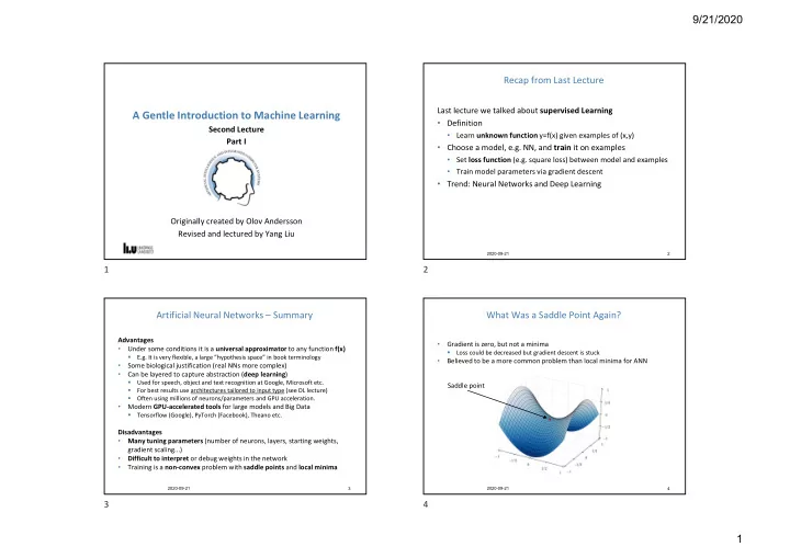
What Was a Saddle Point Again?

2020-09-21 4

• Gradient is zero, but not a minima
• Loss could be decreased but gradient descent is stuck
• Believed to be a more common problem than local minima for ANN

Saddle point

1 2 3 4

9/21/2020 2

Outline of This Lecture

Wrap up supervised learning

• Pitfalls & Limitations
• SL for Learning To Act

Reinforcement Learning

• Introduction
• Q‐Learning (lab5)

Next lecture

• Deep learning, a closer look

2020-09-21 5

Machine Learning Pitfall ‐ Overfitting

• Models can overfit if you have too many parameters in relation to the

training set size.

• Example: 9th degree polynomial regression model (10 parameters) on 15

data points:

• This is not a local minima during training, it is the best fit possible on the

given training examples!

• The trained model captured ”noise” in data, variations independent of f(x)

2020-09-21 6

Green: True function (unknown) Blue: Training examples (noisy!) Red: Trained model (Bishop, 2006)

Overfitting – Where Does the Noise Come From?

• Noise are small variations in the data due to ignored or unknown

variables, that cannot be predicted via chosen feature vector x

• Example: Predict the temperature based on season and time‐of‐day. What

about atmospheric changes like a cold front? As they are not included in the model, nor entirely captured by other input features, their variation will show up as seemingly random noise for the model!

• With low proportion of examples vs. model parameters, training can also

mistake the variation that unmodeled variables cause in y as coming from variables x that are included. This is known as “overfitting”.

• Since this x‐>y relationship was merely chance, the model will not generalize

well to future situations

• It is usually impossible to include all variables affecting the target y’s
• Overfitting is important to guard against!

2020-09-21 7

Overfitting ‐ Demo

• See the interactive example of ANN training again

http://playground.tensorflow.org/

• 2D input x ‐> 1D y (binary classification or regression)

Exercise:

• Pick the bottom‐left data set, two (Gaussian) clusters
• Make a flexible network, e.g. 2 hidden layers w/ 8 neurons each
• Set ”Ratio of training to test data” to 10%
• Max out noise
• Train for a while, can adjust ”learning rate”
• Compare result to ”Show test data”
• How well does this model generalize?

Up next: How do we fix it?

2020-09-21 8

5 6 7 8

9/21/2020 3

Model Selection – Choosing Between Models

• In conclusion, we want to avoid unnecessarily complex models
• This is a fairly general concept throughout science and is often referred to

as Ockham’s Razor:

“Pluralitas non est ponenda sine necessitate” ‐Willian of Ockham “Everything should be kept as simple as possible, but no simpler.” ‐Albert Einstein (paraphrased)

• There are several mathematically principled ways to penalize model

complexity during training, e.g. regularization, which we will not cover here.

• A simple approach is to use a separate validation set with examples that

are only used for evaluating models of different complexity.

2020-09-21 9

Model Selection – Hold‐out Validation

• This is called a hold‐out validation set as we keep the data away from the

training phase

• Measuring performance (loss) on such a validation set is a better metric of

actual generalization error to unseen examples

• With the validation set we can compare models of different complexity to

select the one which generalizes best.

• Examples could be polynomial models of different order, the number of

neurons or layers in an ANN etc.

2020-09-21 10

Validation Set Training Set Given example data:

Measuring Final Generalization Error

• We have seen that having a validation set will lead to a more

accurate estimation of generalization error to use for model selection

• However, by extensively using the validation set for model

selection we can also to contaminate it (overfitting model against the data in the validation set)

• To combat this one usually sets aside a separate test set
• This test set is not used during training or model selection
• It is basically locked away in a safe and only brought out in the end

to get a fair estimate of final generalization error

Validation Set Training Set Given example data:

2020-09-21 11

Test Set Best choice Overfitting

Model Selection – Selection Strategy

• As the number of parameters increases, the size of the hypothesis space

also increases, allowing a better fit to training data

• However, at some point it is sufficiently flexible to capture the underlying
• patterns. Any more will just capture noise, leading to worse generalization

to new examples!

• Do we need to train and test many

models of different complexity?

• Various tricks to avoid this

2020-09-21 12

Example: Prediction error vs. model complexity

• ver many (simulated) data sets. (Hastie et al.,

2009) Red: Validation set (generalization) error Blue: Training set error

9 10 11 12

9/21/2020 4

Early Stopping: Model Complexity Trick with Neural Networks

• Training neural networks tends to progress from simple functions to more

complex ones

• This comes from initializing the parameter values w close to zero
• Remember, a neuron’s output = g(w*x)
• Common activation functions g (e.g. sigmoid) are linear around zero
• This makes the NN effectively ”start out” as a linear model
• Early stopping NN trick: Can make a model complexity vs. validation loss

curve while training, stop when validation error starts increasing Exercise: Back to the NN demo app

• Observe ”test loss” plot
• Reset network
• Train again, but keep an eye on test loss
• Try to pause at low test loss
• Can adjust ”learning rate”

2020-09-21 13

Stop training here!

Limitations of Supervised Learning

• We noted earlier that the first phase of learning is traditionally to select

the ”features” to use as input vector x to the algorithm

• In the spam classification example we restricted ourselves to a set of

relevant words (bag‐of‐words), but even that could be thousands

• Even for such binary features we would have needed O(2#features) examples

to cover all possible combinations

• In a continuous feature space, there might be a difficult non‐linear case

where we need a grid with 10 examples along each feature dimension, which would require O(10#features) examples.

2020-09-21 14

(Bishop, 2006)

The Curse of Dimensionality

• This is known as the curse of dimensionality and also applies to

reinforcement learning as we shall see later

• However, this is a worst‐case scenario.
• The true amount of data needed for supervised learning depends on the

model and the complexity of the function we are trying to learn

• Deep learning may overcome this since it can capture hierarchical abstractions
• Usually, learning works rather well even for many features
• However, selecting features and a model that reflect problem structure can be

the difference between success and failure

• Even for neural networks, e.g. Convolutional NNs

2020-09-21 15

Some Application Examples of Dimensionality

Computer Vision – Object Recognition

• One HD image can be 1920x1080 = 2 million pixels
• If each pixel is naively treated as one dimension, learning to classify

images (or objects in them) can be a million‐dimensional problem.

• Much of computer vision involves clever ways to extract a small set of

descriptive features from images (edges, contrasts)

• Recently deep convolutional networks dominate most benchmarks

Data Mining – Product models, shopping patterns etc

• Can be anything from a few key features to millions
• Can often get away with using linear models, for the very high‐

dimensional cases there are few easy alternatives, although NNs gaining popularity

2020-09-21 16

13 14 15 16

9/21/2020 5

Some Application Examples of Dimensionality II

Robotics

• For perception, see the computer vision considerations, but need real‐time

performance

• For control, e.g. learning robot motion
• Moderate dimension, but non‐linear and require high accuracy (robustness)
• Ground robots have at least a handful dimensions
• Air vehicles (UAVs) have at least a dozen dimensions
• Humanoid robots have at least 30‐60 dimensions
• The human body is said to have over 600 muscles
• Traditionally uses tailored models based on e.g. physics approximations
• Learning is gaining ground but data not as easy to collect as robots can break (or

hurt somebody)

2020-09-21 17

From Supervised to Reinforcement Learning ‐ Learning How to Act

• Can we use supervised learning to learn how to act?
• E.g. engineering robot behavior can be fragile and time consuming
• Things humans do without thinking require extremely detailed

instructions for a robot. Even robust locomotion is hard.

Humorous reminder from IEEE Spectrum: The DARPA 2015 Humanoid Challenge “Fail Compilation”

18

Learning How to Act

• Yes, one can learn a mapping from problem state (e.g. position) to action
• As in all supervised learning, this requires a teacher
• Sometimes called ”imitation learning”
• However, supervised learning with robots can get tedious as providing

examples of correct behaviour is difficult to automate

• Can we remove the human from the loop?

1. An automated teacher like a planning or optimal control algorithm can generate supervised examples if it as a model of the environment

• Mordatch et al, https://www.youtube.com/watch?v=IxrnT0JOs4o
• Our research w/ real nano‐quadcopters (deep ANN on‐board the microcontroller)

2. Reinforcement learning attempts to generalize this to learning from scratch in completely unknown environments

2020-09-21 19

17 18 19

A Gentle Introduction to Machine Learning

Part II - Reinforcement Learning Originally created by Olov Andersson Revised and lectured by Yang Liu

Artificial Intelligence and Integrated Computer Systems Department of Computer and Information Science Linköping University

1 (AIICS, IDA, LiU) Reinforcement Learning 1 / 15

Introduction to Reinforcement Learning

Remember:

In Supervised Learning agents learn to act given examples of correct choices.

What if an agent is given rewards instead? Examples:

In a game of chess, the agent may be rewarded when it wins. A soccer playing agent may be rewarded when it scores a goal. A helicopter acrobatics agent may be rewarded if it performs a loop. A pet agent may be given a reward if it fetches its masters slippers.

These are all examples of Reinforcement Learning, where the agent itself figures out how to solve the task.

1 (AIICS, IDA, LiU) Reinforcement Learning 2 / 15

Defining the domain

How do we formally define this problem? An agent is given a sensory input consisting of: State s ∈ S (from type problem domain) Reward R(s) ∈ R (our way to encode objective in domain) It should pick an output Action a ∈ A (based on type of robot/agent) It wants to learn the "best" action for each state.

1 (AIICS, IDA, LiU) Reinforcement Learning 3 / 15

What do we need to solve?

An example domain... S = {squares} A = {N,W,S,E} R(s) = 0 except for the two terminal states on the right Considerations:

It may not know the effect of actions yet p(s′|s, a) It may not know the rewards R(s) in all states yet Reward will be zero for all actions in all states not adjacent to the two terminal states. Need to consider reward of future moves!

1 (AIICS, IDA, LiU) Reinforcement Learning 4 / 15

Rewards and Utility

We define the reward for reaching a state si as R(si) To plan ahead it must look at a sum of rewards over a sequence

• f states R(si+1), R(si+2), R(si+2), ...

This can be formalized as the utility U for the sequence U =

∞

• t=0

γtR(st), where 0 < γ < 1 (1) Where γ < 1 is the discount factor making the utility finite even for infinite sequences. A low γ makes the agent very short-sighted and greedy, while a gamma close to one makes it very patient (γ ≈ planning horizon).

1 (AIICS, IDA, LiU) Reinforcement Learning 5 / 15

The Policy Function

We now have a utility function for a sequence of states ...but the sequence of states depends on the actions taken! We need one last concept, a policy function π(s) decides which action to take in each state a = π(s) (2) Clearly, a good policy function is what we set out to find

Figure: A policy function maps states to actions (arrows). Note it’s not necessarily optimal.

1 (AIICS, IDA, LiU) Reinforcement Learning 6 / 15

Examples of optimal policies for different R(s)

Assuming random transition function (for each direction):

1 (AIICS, IDA, LiU) Reinforcement Learning 7 / 15

How to find such an optimal policy?

There are two different philosophies for solving these problems Model-based reinforcement learning

Learn R(s) and f(s, a) = s′ using supervised learning. Solve a (probabilistic) planning problem using an algorithm like value iteration (see book, not included in this course).

Model-free reinforcement learning

Use an iterative algorithm that implicitly both adapts to the environment and solves the planning problem. Q-learning is a popular such algorithm that has a very simple

• implementation. (lab5)

1 (AIICS, IDA, LiU) Reinforcement Learning 8 / 15

Q-Learning

In Q-learning, all we need to keep track of is the "Q-table" Q(s, a), a table of estimated utilities for taking action a in state s. If we knew the long-term value of an action, solving the planning problem to compute policy π(s) reduces to just taking the best action in the Q-table: maxα∈A Q(s, a) Turns out one can learn the Q-table for the optimal policy by applying an iterative update rule on the Q-table as the agent moves In a simpler deterministic world (no randomness) this is: Q(s, a) ← R(s) + γ max

a′∈A Q(s′, a′)

(3) where γ is the discount factor. An intuition is to remember that Q-value = estimated utility = sum

• f rewards. We can define the Q-value for the optimal policy

recursively as the immediate reward, plus the discounted best Q-value in the next state (compare Eq.(1)). Then just iterate!

1 (AIICS, IDA, LiU) Reinforcement Learning 9 / 15

Q-Learning II - Final Version

The full update rule, also accounting for randomness in state transitions is: Q(s, a) ← Q(s, a) + α(R(s) + γ max

a′∈A Q(s′, a′) − Q(s, a))

(4) where α is the learning rate and γ is the discount factor. Each time an agent moves, the Q-values are updated by a small factor α towards the Q-value of the next state, acting as an average over all possible (now random) next states for an action. For full proof, see the book (not needed for exam). NOTE: Approximations of the state space, like the discretization in lab5, can cause apparent randomness from just observing the approximate state.

1 (AIICS, IDA, LiU) Reinforcement Learning 10 / 15

The Q-table Update - An Example

Where actions are N,E,S,W (North = up) and γ = 0.9. For simplicity the agent repeatedly executes the actions above, ending each episode in the terminal +1 state and restarting. Transitions are deterministic so we use learning rate α = 1. Begin by initializing all terminal Q(sT, ∗) = reward, all other Q(s, a) = 0 For each step the agent updates Q(s,a) for the previous state/action: Q(s, a) ← Q(s, a) + α(R(s) + γ max

a′∈A Q(s′, a′) − Q(s, a))

After a while the Q-values will converge to the true utility

1 (AIICS, IDA, LiU) Reinforcement Learning 11 / 15

The Q-Learning Update - An Example

Q(s, a) ← Q(s, a) + α(R(s) + γ max

a′∈A Q(s′, a′) − Q(s, a))

First run (clarified): Q(s3,3, E) = 0 + 1 · (0 + 0.9 · max(1, 1, 1, 1) − 0) = 0.9. (Remember, all action Q-vals for terminal s4,4 initialized to +1) Second run: Q(s3,2, N) = 0 + 1 · (0 + 0.9 max(0, 0.9, 0, 0) − 0) = 0.81, Q(s3,3, E) = 0.9 (unchanged due to learning rate α = 1) Third run: Q(s3,1, N) = 0 + 1 · (0 + 0.9 max(0.81, 0, 0, 0) − 0) = 0.729, Q(s3,2, N) = 0.81, Q(s3,3, E) = 0.9 (both unchanged). And so on...

1 (AIICS, IDA, LiU) Reinforcement Learning 12 / 15

Action selection while learning: Exploration

That was assuming fixed actions. The agent should ideally pick the action with highest utility (Q-value). However, always taking the highest estimated utility action while still learning will get the agent stuck in a sub-optimal policy. In the previous example, once the Q-table has been updated all the way to the start position, following that path will always be the

• nly non-zero (and therefore best) choice.

The agent needs to balance taking the currently highest Q-value actions with exploring the other options! ǫ-greedy is an exploration strategy that takes a random move with some probability, so it (eventually) tests all state-action

• combinations. Without exploration, Q-learning is greedy by picking

the highest value action in Q-table, which means some state-actions are never tested. With simple ǫ-greedy strategy it is only greedy with probability ǫ, and does random moves with probability 1-ǫ.

1 (AIICS, IDA, LiU) Reinforcement Learning 13 / 15

Curse of Dimensionality for Q-Learning

Need to discretize continuous state and action spaces. The Q-table will grow exponentially with their dimension! Workaround: Approximate Q-table by supervised learning.

"Fitted" Q-iteration. See Q-table as unknown f(x), (state,action) as examples of input x, and the Q-value after update as example

• utput y. Can learn this from new examples as the agent moves.

If approximation generalizes well, we get large gains in scalability. Use deep learning → deep reinforcement learning

Deep ANN was used for the video game example (plus some tricks) Google’s Go champion combines several approaches, deep convolutional nets for approximating the game board, a tree-search planning approach for updating utilities and more...

Caveat: Non-linear approximations may impede convergence.

1 (AIICS, IDA, LiU) Reinforcement Learning 14 / 15

Q-Learning - Final Words

Implementation is very simple, having no model of the environment.

It only needs a table of Q(s,a) values!

Once the Q(s,a) function has converged, the optimal policy π∗(s) is simply the action with highest utility in the table for each s Technically the learning rate α actually needs to decrease over time for perfect convergence. Q-learning must also be combined with exploration Q-learning requires very little computational overhead per step The curse of dimensionality: The Q-table grows exponentially with

• dimension. A good approximation can avoid this.

Model-free methods may require more interactions with the world than model-based, and much more than a human.

1 (AIICS, IDA, LiU) Reinforcement Learning 15 / 15