6.869 Model-based Vision Topics: Advances in Computer Vision - - PDF document

SLIDE 1

1

1

6.869

Advances in Computer Vision

• Prof. Bill Freeman

Model-based vision

• Hypothesize and test
• Interpretation Trees
• Alignment
• Pose Clustering
• Geometric Hashing

Readings: F&P Ch 18.1-18.5

2

Model-based Vision

Topics:

– Hypothesize and test

• Interpretation Trees
• Alignment

– Interpretation trees – Hypothesis generation methods

• Pose clustering
• Invariances
• Geometric hashing

– Verification methods

3

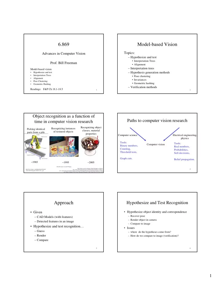
Object recognition as a function of time in computer vision research

~1985 ~1995 ~2005 Picking identical parts from a pile Recognizing instances

• f textured objects

Recognizing object classes, material properties

http://images.google.com/imgres?imgurl=http://www.displayit- info.com/food/images/desserts/2131.JPG&imgrefurl=http://www.displayit- info.com/food/dessert6.html&h=504&w=501&sz=181&tbnid=FXJATGzVyA4J:&tbnh=128&tbnw=127&st art=13&prev=/images%3Fq%3Dice%2Bcream%2Bsundae%26hl%3Den%26lr%3D%26sa%3DG dollarfifty.tripod.com/ pho/004lg.jpg http://www.fanuc.co.jp/en/product/robot/rob

• tshow2003/image/m-16ib20_3dv_e.gif

4

Paths to computer vision research

Computer vision Computer science Electrical engineering, physics Tools: Binary numbers, Counting, Threshold tests, Graph cuts. Tools: Real numbers, Probabilities, Soft decisions, Belief propagation.

5

Approach

• Given

– CAD Models (with features) – Detected features in an image

• Hypothesize and test recognition…

– Guess – Render – Compare

6

Hypothesize and Test Recognition

• Hypothesize object identity and correspondence

– Recover pose – Render object in camera – Compare to image

• Issues

– where do the hypotheses come from? – How do we compare to image (verification)?

SLIDE 2

2

7

Features?

• Points

but also,

• Lines
• Conics
• Other fitted curves
• Regions (particularly the center of a region, etc.)
• More descriptive local features (eg work by

Schmid and Lowe). “…of intermediate complexity, which

means that they are distinctive enough to determine likely matches in a large database of features, but are sufficiently local to be insensitive to clutter and occlusion”. (Lowe, CVPR01)

8

How to generate hypotheses?

• Brute force

– Construct a correspondence for all object features to every correctly sized subset of image points – Expensive search, which is also redundant. – L objects with N features – M features in image – O(LMN) !

9

Brute force method

L models image A B C Try all M image feature points for a model point, Then try all M-1 remaining image feature points for another model point, then all M-2 for the next, etc. M * (M-1) * (M-2) …* (M-N+1) for each of L models= O(LMN )

M pts N pts

10

Ways around that combinatorial explosion

• Add geometric constraints to prune search, leading

to interpretation tree search

• Try subsets of features (frame groups)…

11

Frame groups

• A group of features that can yield a camera hypothesis.
• If you know the intrinsic parameters of your camera, then

these are the set of features needed to specify the object’s pose relative to the camera.

• With a perspective camera model, known intrinsic camera

parameters, some frame groups are:

3 points Trihedral vertex, and a point (for scale) Dihedral vertex, and a point

12

Adding constraints

• Correspondences between image features and

model features are not independent.

• A small number of good correspondences yields a

reliable pose estimation --- the others must be consistent with this.

• Generate hypotheses using small numbers of

correspondences (e.g. triples of points for a calibrated perspective camera, etc., etc.)

SLIDE 3

3

13

Pose consistency / Alignment

• Given known camera type in some

unknown configuration (pose)

– Hypothesize configuration from set of initial features – Backproject – Test

14

Rendering an object into the image

Perspective camera

15

Rendering an object into the image

i i

AP p Π =

Affine camera ⎟ ⎟ ⎟ ⎠ ⎞ ⎜ ⎜ ⎜ ⎝ ⎛ = Π 1 1 1

⎟ ⎟ ⎟ ⎟ ⎟ ⎠ ⎞ ⎜ ⎜ ⎜ ⎜ ⎜ ⎝ ⎛ = 1

23 22 21 20 13 12 11 10 03 02 01 00

a a a a a a a a a a a a A

Rendering ith 3d pt to 2d image position Orthographic camera General affine transformation

16

A frame group for an affine camera model

i i

AP p Π =

Affine camera

⎟ ⎟ ⎠ ⎞ ⎜ ⎜ ⎝ ⎛ + + + + + + = ⎟ ⎟ ⎠ ⎞ ⎜ ⎜ ⎝ ⎛

3 13 2 12 1 11 10 3 03 2 02 1 01 00 1 i i i i i i i i i i

P a P a P a P a P a P a P a P a p p

Rendering ith 3d pt to 2d image position

⎟ ⎟ ⎟ ⎠ ⎞ ⎜ ⎜ ⎜ ⎝ ⎛ = Π 1 1 1

⎟ ⎟ ⎟ ⎟ ⎟ ⎠ ⎞ ⎜ ⎜ ⎜ ⎜ ⎜ ⎝ ⎛ = 1

23 22 21 20 13 12 11 10 03 02 01 00

a a a a a a a a a a a a A Orthographic camera General affine transformation Relating observed 2-d positions to 3-d model positions Need at least 4 points in general position to determine the affine camera parameters. (Note: only the 1st 2 rows of A contribute to the projection, so we only need to estimate them.)

17

Alignment algorithm

18

SLIDE 4

4

19

More than 1 object in image

• Require same intrinsic camera parameters

for each object.

20

Model-based Vision

Topics:

– Hypothesize and test

• Interpretation Trees
• Alignment

– Interpretation trees – Hypothesis generation methods

• Pose clustering
• Invariances
• Geometric hashing

– Verification methods

21

Interpretation Trees

• Tree of possible model-image feature assignments
• Depth-first search
• Prune when unary (binary, …) constraint violated

– length – area – orientation (a,1) (b,2) … …

22

Interpretation Trees

[ A.M. Wallace. 1988. ]

“Wild cards” handle spurious image features

http://faculty.washington.edu/cfolson/papers/pdf/icpr04.pdf 23

Model-based Vision

Topics:

– Hypothesize and test

• Interpretation Trees
• Alignment

– Interpretation trees – Hypothesis generation methods

• Pose clustering
• Invariances
• Geometric hashing

– Verification methods

24

• How does the hypothesize and test method

fail?

– False matches – Too many hypotheses to consider

• To add robustness and efficiency, use other

heuristics to select candidate object poses

SLIDE 5

5

25

Pose clustering

• Each model leads to many correct sets of

correspondences, each of which has the same pose

• Vote on object pose, in an accumulator array (per
• bject)
• This is a computer science approach to doing a

more probabilistic thing: treating each set of feature observations as statistically independent and multiplying together their probabilities of

• ccurrence to obtain a likelihood function.

26

Pose Clustering

27

Two models used in an early pose clustering system

28

Pose clustering

Problems

– Clutter may lead to more votes than the target! – Difficult to pick the right bin size

Confidence-weighted clustering

– See where model frame group is reliable (visible!) – Downweight / discount votes from frame groups at poses where that frame group is unreliable… – Again, we can make this more precise in a probabilistic framework later.

29

pick feature pair dark regions show reliable-pose-estimate views of those features over the viewing sphere

30

Test image, with edge points marked

SLIDE 6

6

31

Image with edges of found models overlaid

32 33

Detected airplanes, rerendered at their detected

• poses. (Note mis-estimated

pose of plane on runway.)

34

A more recent pose/view clustering example

• “Local feature view clustering for 3D object recognition”,

by David Lowe (see his web page for copy).

• Schmid, Lowe incorporate “super-features”, point

features with robust local image descriptors

35

Detecting 0.1% inliers among 99.9% outliers?

• Example: David Lowe’s SIFT-based Recognition system
• Goal: recognize clusters of just 3 consistent features

among 3000 feature match hypotheses

• Approach

– Vote for each potential match according to model ID and pose – Insert into multiple bins to allow for error in similarity approximation – Using a hash table instead of an array avoids need to form empty bins or predict array size

[Lowe]

36

Lowe’s Model verification step

• Examine all clusters with at least 3 features
• Perform least-squares affine fit to model.
• Discard outliers and perform top-down check for

additional features.

• Evaluate probability that match is correct

– Use Bayesian model, with probability that features would arise by chance if object was not present – Takes account of object size in image, textured regions, model feature count in database, accuracy of fit (Lowe, CVPR 01)

[Lowe]

SLIDE 7

7

37

Solution for affine parameters

• Affine transform of [x,y] to [u,v]:
• Rewrite to solve for transform parameters:

[Lowe]

38

Models for planar surfaces with SIFT keys:

[Lowe]

39

Planar recognition

• Planar surfaces can be

reliably recognized at a rotation of 60° away from the camera

• Affine fit approximates

perspective projection

• Only 3 points are

needed for recognition

[Lowe]

40

3D Object Recognition

• Extract outlines

with background subtraction

[Lowe]

41

3D Object Recognition

• Only 3 keys are

needed for recognition, so extra keys provide robustness

• Affine model is no

longer as accurate

[Lowe]

42

Recognition under occlusion

[Lowe]

SLIDE 8

8

43

Model-based Vision

Topics:

– Hypothesize and test

• Interpretation Trees
• Alignment

– Interpretation trees – Hypothesis generation methods

• Pose clustering
• Invariances
• Geometric hashing

– Verification methods

44

Geometric Invariant recognition

• It’s a pain to compute some many pose or

correspondences for verification. So insert a pruning step that is invariant to camera/object pose parameters.

• Affine invariants

– Planar invariants – Geometric hashing

• Projective invariants

– Determinant ratio

• Curve invariants

45

Invariance

• There are geometric properties that are invariant to

camera transformations

• Easiest case: view a plane object in scaled
• rthography.
• Assume we have three base points P_i on the
• bject

– then any other point on the object can be written as

P

k = P 1 + µka P 2 − P 1

( )+ µkb P

3 − P 1

( )

46

Invariance

• Now image points are obtained by multiplying

by a plane affine transformation, so

pk = AP

k

= A P

1 + µka P 2 − P 1

( )+ µkb P

3 − P 1

( )

( )

= p1 + µka p2 − p1

( )+ µkb p3 − p1 ( )

47

Invariance

Given the base points in the image, read off the µ values for the object

– they’re the same in object and in image --- invariant – search correspondences, form µ’s and vote

pk = AP

k

= A P

1 + µka P 2 − P 1

( )+ µkb P

3 − P 1

( )

( )

= p1 + µka p2 − p1

( )+ µkb p3 − p1 ( )

P

k = P 1 + µka P 2 − P 1

( )+ µkb P

3 − P 1

( )

48

Indexing

• Operation that lets you select the model

from a menu of possible ones, before you need to find the pose and verify.

http://www.tnt.uni-hannover.de/project/imgint/industrial/3dpos/3DLageerkennung.gif

SLIDE 9

9

49

Indexing with invariants

• Generalize to heterogeneous geometric

features

• Groups of features with identity

information invariant to pose – invariant bearing groups

50

Projective invariants

• Projective invariant for coplanar points
• Perspective projection of coplanar points

is a plane perspective transform:

p=MP p=AP, with 3x3 A

• determinant ratio of 5 point tuples is

invariant

det pi pj pk

[ ]

( )

det pi pl pm

[ ] ( )

det pi pj pl

[ ]

( )

det pi pk pm

[ ] ( )

51

det pi pj pk

[ ]

( )

det pi pl pm

[ ] ( )

det pi pj pl

[ ]

( )

det pi pk pm

[ ] ( )

= det APiAP jAP k

[ ]

( )

det APiAPlAP m

[ ] ( )

det AP iAP jAPl

[ ]

( )

det AP

iAP kAPm

[ ] ( )

= det A P

iPjP k

[ ]

( )

det A P

iP lP m

[ ] ( )

det A P

iPjP l

[ ]

( )

det A P

iP kP m

[ ] ( )

= det A

( )

2

( )

det A

( )

2

( )

det P

iPjP k

[ ]

( )

det P

iP lP m

[ ] ( )

det P

iPjP l

[ ]

( )

det P

iP kP m

[ ] ( )

= det P

iPjP k

[ ]

( )

det P

iP lP m

[ ] ( )

det P

iPjP l

[ ]

( )

det P

iP kP m

[ ] ( )

52

Geometric Hashing

• Objects are represented as sets of “features”
• Preprocessing:

– For each tuple b of features, compute location (µ) of all other features in basis defined by b – Create a table indexed by (µ) – Each entry contains b and object ID

• S. Rusinkiewicz

[http://www.cs.princeton.edu/courses/archive/fall03/cs597D/lectures/rigid_registration.pdf]

53

Geometric hashing

;1,5,6 ;4,5,7 ;4,5,7 ;1,3,4/ ;1,5,6 ;1,3,4 ;2,3,6 D A A A D D B ⎛ ⎞ ⎜ ⎟ ⎜ ⎟ ⎜ ⎟ ⎜ ⎟ ⎝ ⎠

1

µ

2

µ A B C

1 2 3 4 5 6 7 8

Models Hash table

1 2 3 4 5 6 7 8 1 2 3 4 5 6 54

GH: Identification

• Find features in target image
• Choose an arbitrary basis b’
• For each feature:

– Compute (µ’) in basis b’ – Look up in table and vote for (Object, b)

• For each (Object, b) with many votes:

– Compute transformation that maps b to b’ – Confirm presence of object, using all available features

• S. Rusinkiewicz

[http://www.cs.princeton.edu/courses/archive/fall03/cs597D/lectures/rigid_registration.pdf]

SLIDE 10

10

55

Geometric Hashing

Wolfson and Rigoutsos, Geometric Hashing, an Overview, 1997

[http://www.cs.princeton.edu/courses/archive/fall03/cs597D/lectures/rigid_registration.pdf]

56

Basis Geometric Hashing

Wolfson and Rigoutsos, Geometric Hashing, an Overview, 1997

[http://www.cs.princeton.edu/courses/archive/fall03/cs597D/lectures/rigid_registration.pdf]

57

Geometric Hashing

Wolfson and Rigoutsos, Geometric Hashing, an Overview, 1997

[http://www.cs.princeton.edu/courses/archive/fall03/cs597D/lectures/rigid_registration.pdf]

58

==b

59

Tangent invariance

• Incidence is preserved despite transformation
• Transform four points above to unit square:

measurements in this canonical frame will be invariant to pose.

M-curve construction

60

SLIDE 11

11

61

From Rothwell et al, CVPR 92.

Recognizing planar objects using invariants.

Input image Edge points fitted with lines or conics Objects that have been recognized and verified.

62

Verification

• Edge score

– are there image edges near predicted object edges? – very unreliable; in texture, answer is usually yes

• Oriented edge score

– are there image edges near predicted object edges with the right

• rientation?

– better, but still hard to do well (see next slide)

• Texture largely ignored [Forsythe]

– e.g. does the spanner have the same texture as the wood?

63

52% of the edge points for this candidate object were verified in the wood texture underneath.

Rothwell et al, CVPR 92.

64

Algorithm Sensitivity

Grimson and Huttenlocher, 1990

• Geometric Hashing

– A relatively sparse hash table is critical for good performance – Method is not robust for cluttered scenes (full hash table) or noisy data (uncertainty in hash values)

• Generalized Hough Transform

– Does not scale well to multi-object complex scenes – Also suffers from matching uncertainty with noisy data

[http://www.cs.princeton.edu/courses/archive/fall03/cs597D/lectures/rigid_registration.pdf]

65

Comparison to template matching

• Costs of template matching

– 250,000 locations x 30 orientations x 4 scales = 30,000,000 evaluations – Does not easily handle partial occlusion and other variation without large increase in template numbers – Viola & Jones cascade must start again for each qualitatively different template

• Costs of local feature approach

– 3000 evaluations (reduction by factor of 10,000) – Features are more invariant to illumination, 3D rotation, and object variation – Use of many small subtemplates increases robustness to partial

• cclusion and other variations

[Lowe]

66

Model-based Vision

Topics:

– Hypothesize and test

• Interpretation Trees
• Alignment

– Hypothesis generation methods

• Pose clustering
• Invariances
• Geometric hashing

– Verification methods