
SLIDE 1
1/28/16 CMPS 6640/4040 Computational Geometry 1
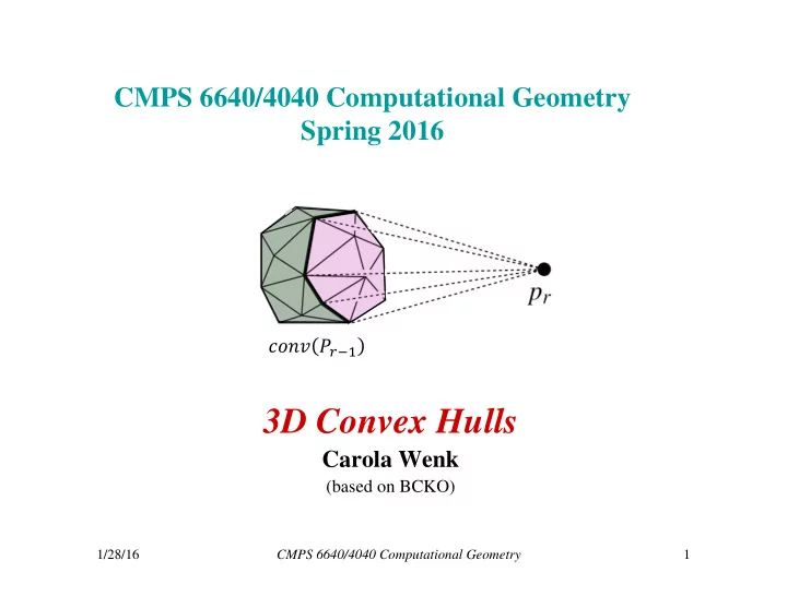
CMPS 6640/4040 Computational Geometry Spring 2016
3D Convex Hulls
Carola Wenk
(based on BCKO)
3D Convex Hulls Carola Wenk (based on BCKO) 1/28/16 CMPS - - PowerPoint PPT Presentation
CMPS 6640/4040 Computational Geometry Spring 2016 3D Convex Hulls Carola Wenk (based on BCKO) 1/28/16 CMPS 6640/4040 Computational Geometry 1 3D CH: Problem Statement Images from http://xlr8r.info/ compute
1/28/16 CMPS 6640/4040 Computational Geometry 1
(based on BCKO)
Images from http://xlr8r.info/
be a random permutation of the remaining
by inserting into
, then
, separated by the horizon.
is visible from
lies in , where is the plane containing ,
is the open halfspace that does not contain
, as a DCEL. The vertices are 3D points.
and for
in linear time
incident to in convP
and
||
Face can only be deleted if it has been created. Delete at most once
∈
and arc creation
|
proof in book
|
|
Total degree of , … , is at least 12
is / .
/