3. Examples Ancient Egyptian Multiplication Example on how to show - PowerPoint PPT Presentation

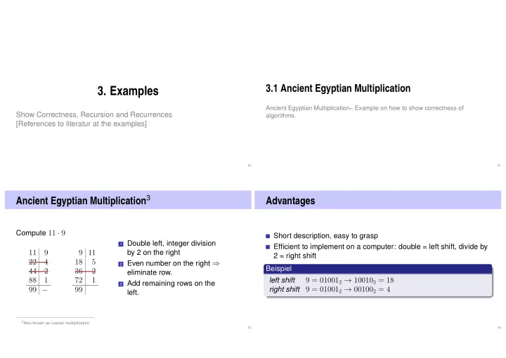
3.1 Ancient Egyptian Multiplication 3. Examples Ancient Egyptian Multiplication– Example on how to show correctness of Show Correctness, Recursion and Recurrences algorithms. [References to literatur at the examples] 60 61 Ancient Egyptian Multiplication 3 Advantages Compute 11 · 9 Short description, easy to grasp 1 Double left, integer division Efficient to implement on a computer: double = left shift, divide by 11 9 9 11 by 2 on the right 2 = right shift 22 4 18 5 2 Even number on the right ⇒ Beispiel 44 2 36 2 eliminate row. 9 = 01001 2 → 10010 2 = 18 88 1 72 1 left shift 3 Add remaining rows on the 99 − 99 right shift 9 = 01001 2 → 00100 2 = 4 left. 3 Also known as russian multiplication 62 63

Questions The Essentials If b > 1 , a ∈ ❩ , then: For which kind of inputs does the algorithm deliver a correct � result (in finite time)? 2 a · b falls b gerade, 2 a · b = How do you prove its correctness? a + 2 a · b − 1 falls b ungerade. 2 What is a good measure for Efficiency? 64 65 Termination Recursively, Functional   a falls b = 1 , a falls b = 1 ,     2 a · b f (2 a, b a · b = falls b gerade, f ( a, b ) = 2 ) falls b gerade, 2   a + 2 a · b − 1 a + f (2 a, b − 1   falls b ungerade. 2 ) falls b ungerade. 2 66 67

Implemented as a function Correctnes: Mathematical Proof // pre: b>0  // post: return a ∗ b a if b = 1 ,  int f(int a, int b){  f (2 a, b f ( a, b ) = 2 ) if b even, if(b==1)  return a; a + f (2 a · b − 1  2 ) if b odd. else if (b%2 == 0) return f(2 ∗ a, b/2); else return a + f(2 ∗ a, (b − 1)/2); Remaining to show: f ( a, b ) = a · b for a ∈ ❩ , b ∈ ◆ + . } 68 69 Correctnes: Mathematical Proof by Induction [Code Transformations: End Recursion] ∀ b ∈ ◆ + . Let a ∈ ❩ , to show f ( a, b ) = a · b The recursion can be writen as end recursion Base clause: f ( a, 1) = a = a · 1 // pre: b>0 ∀ 0 < b ′ ≤ b Hypothesis: f ( a, b ′ ) = a · b ′ // post: return a ∗ b // pre: b>0 ∀ 0 < b ′ ≤ b ! // post: return a ∗ b Step: f ( a, b ′ ) = a · b ′ int f(int a, int b){ ⇒ f ( a, b + 1) = a · ( b + 1) int f(int a, int b){ if (b==1)  if (b==1) return a; 0 < ·≤ b  � �� �  return a; int z=0;  b + 1  i.H.  f (2 a, ) = a · ( b + 1) if b > 0 odd, else if (b%2 == 0) if (b%2 != 0){  2 f ( a, b + 1) = return f(2 ∗ a, b/2); −− b; b i.H. else z=a;  a + f (2 a, ) = a + a · b if b > 0 even.   2 return a + f(2 ∗ a, (b − 1)/2);  }   ���� } return z + f(2 ∗ a, b/2); 0 < · <b } � 70 71

[Code-Transformation: End-Recursion ⇒ Iteration] [Code-Transformation: Simplify] int f(int a, int b) { int f(int a, int b) { int res = 0; int res = 0; // pre: b>0 // pre: b>0 while (b != 1) { while (b != 1) { // post: return a ∗ b // post: return a ∗ b int z = 0; int z = 0; int f(int a, int b){ int f(int a, int b) { if (b % 2 != 0){ if (b % 2 != 0){ if (b==1) int res = 0; −− b; −− b; Teil der Division return a; while (b > 0) { z = a; z = a; Direkt in res int z=0; if (b % 2 != 0) } } if (b%2 != 0){ res += a; res += z; res += z; −− b; a ∗ = 2; a ∗ = 2; // neues a a ∗ = 2; z=a; b /= 2; b /= 2; // neues b b /= 2; } } } } return z + f(2 ∗ a, b/2); return res ; res += a; // Basisfall b=1 res += a; in den Loop } } return res ; return res ; } } 72 73 Correctness: Reasoning using Invariants! Conclusion // pre: b>0 // post: return a ∗ b The expression a · b + res is an invariant int f(int a, int b) { Sei x := a · b . int res = 0; Values of a , b , res change but the invariant remains basically here: x = a · b + res while (b > 0) { unchanged: The invariant is only temporarily discarded by if (b % 2 != 0){ some statement but then re-established. If such short if here x = a · b + res ... res += a; statement sequences are considered atomiv, the value remains −− b; ... then also here x = a · b + res indeed invariant } b even In particular the loop contains an invariant, called loop invariant a ∗ = 2; b /= 2; and it operates there like the induction step in induction proofs. here: x = a · b + res } here: x = a · b + res und b = 0 Invariants are obviously powerful tools for proofs! return res; Also res = x . } 74 75

[Further simplification] [Analysis] // pre: b>0 // post: return a ∗ b // pre: b>0 // pre: b>0 Ancient Egyptian Multiplication corre- int f(int a, int b) { // post: return a ∗ b // post: return a ∗ b sponds to the school method with int res = 0; int f(int a, int b) { radix 2 . int f(int a, int b) { while (b > 0) { int res = 0; int res = 0; if (b % 2 != 0){ while (b > 0) { 1 0 0 1 × 1 0 1 1 while (b > 0) { res += a; res += a ∗ (b%2); 1 0 0 1 (9) res += a ∗ (b%2); −− b; a ∗ = 2; 1 0 0 1 (18) a ∗ = 2; } b /= 2; 1 1 0 1 1 b /= 2; a ∗ = 2; } 1 0 0 1 (72) } b /= 2; return res ; 1 1 0 0 0 1 1 (99) return res ; } } } return res ; } 77 78 Efficiency Question: how long does a multiplication of a and b take? Measure for efficiency Total number of fundamental operations: double, divide by 2, shift, test for “even”, addition 3.2 Fast Integer Multiplication In the recursive and recursive code: maximally 6 operations per call or iteration, respectively [Ottman/Widmayer, Kap. 1.2.3] Essential criterion: Number of recursion calls or Number iterations (in the iterative case) b 2 n ≤ 1 holds for n ≥ log 2 b . Consequently not more than 6 ⌈ log 2 b ⌉ fundamental operations. 79 80

Example 2: Multiplication of large Numbers Observation Primary school: a b c d 6 2 · 3 7 1 4 d · b ab · cd = (10 · a + b ) · (10 · c + d ) 4 2 d · a = 100 · a · c + 10 · a · c 6 c · b + 10 · b · d + b · d 1 8 c · a = 2 2 9 4 + 10 · ( a − b ) · ( d − c ) 2 · 2 = 4 single-digit multiplications. ⇒ Multiplication of two n -digit numbers: n 2 single-digit multiplications 81 82 Improvement? Large Numbers a b c d 6 2 · 3 7 6237 · 5898 = 62 37 · 58 98 1 4 d · b ���� ���� ���� ���� 1 4 d · b a ′ b ′ c ′ d ′ 1 6 ( a − b ) · ( d − c ) Recursive / inductive application: compute a ′ · c ′ , a ′ · d ′ , b ′ · c ′ and 1 8 c · a c ′ · d ′ as shown above. 1 8 c · a = 2 2 9 4 → 3 · 3 = 9 instead of 16 single-digit multiplications. → 3 single-digit multiplications. 83 84

Generalization Analysis Assumption: two numbers with n digits each, n = 2 k for some k . M ( n ) : Number of single-digit multiplications. Recursive application of the algorithm from above ⇒ recursion (10 n/ 2 a + b ) · (10 n/ 2 c + d ) = 10 n · a · c + 10 n/ 2 · a · c equality: + 10 n/ 2 · b · d + b · d � 1 if k = 0 , M (2 k ) = + 10 n/ 2 · ( a − b ) · ( d − c ) 3 · M (2 k − 1 ) if k > 0 . Recursive application of this formula: algorithm by Karatsuba and Ofman (1962). 85 86 Iterative Substition Proof: induction Hypothesis H : M (2 k ) = 3 k . Iterative substition of the recursion formula in order to guess a solution of the recursion formula: Base clause ( k = 0 ) : M (2 0 ) = 3 0 = 1 . M (2 k ) = 3 · M (2 k − 1 ) = 3 · 3 · M (2 k − 2 ) = 3 2 · M (2 k − 2 ) � = . . . = 3 k · M (2 0 ) = 3 k . ! Induction step ( k → k + 1 ) : = 3 · 3 k = 3 k +1 . def H M (2 k +1 ) = 3 · M (2 k ) � 87 88

Comparison Best possible algorithm? Traditionally n 2 single-digit multiplications. We only know the upper bound n log 2 3 . Karatsuba/Ofman: There are (for large n ) practically relevant algorithms that are faster. Example: Schönhage-Strassen algorithm (1971) based on fast M ( n ) = 3 log 2 n = (2 log 2 3 ) log 2 n = 2 log 2 3 log 2 n = n log 2 3 ≈ n 1 . 58 . Fouriertransformation with running time O ( n log n · log log n ) . The best upper bound is not known. Lower bound: n . Each digit has to be considered at least once. Example: number with 1000 digits: 1000 2 / 1000 1 . 58 ≈ 18 . 89 90 Appendix: Asymptotics with Addition and Shifts Appendix: Asymptotics with Addition and Shifts Assumption: n = 2 k , k > 0 For each multiplication of two n -digit numbers we also should take � 2 k − 1 � T (2 k ) = 3 · T + c · 2 k into account a constant number of additions, subtractions and shifts = 3 · (3 · T (2 k − 2 ) + c · 2 k − 1 ) + c · 2 k Additions, subtractions and shifts of n -digit numbers cost O ( n ) = 3 · (3 · (3 · T (2 k − 3 ) + c · 2 k − 2 ) + c · 2 k − 1 ) + c · 2 k Therefore the asymptotic running time is determined (with some = 3 · (3 · ( ... (3 · T (2 k − k ) + c · 2 1 ) ... ) + c · 2 k − 1 ) + c · 2 k c > 1 ) by the following recurrence = 3 k · T (1) + c · 3 k − 1 2 1 + c · 3 k − 2 2 2 + ... + c · 3 0 2 k ≤ c · 3 k · (1 + 2 / 3 + (2 / 3) 2 + ... + (2 / 3) k ) � � 1 � 3 · T 2 n + c · n if n > 1 T ( n ) = Die geometrische Reihe � k i =0 ̺ i mit ̺ = 2 / 3 konvergiert für k → ∞ gegen 1 otherwise 1 1 − ̺ = 3 . Somit T (2 k ) ≤ c · 3 k · 3 ∈ Θ(3 k ) = Θ(3 log 2 n ) = Θ( n log 2 3 ) . 91 92