3.3 Models, Validity, and Satisfiability is valid in A under - - PowerPoint PPT Presentation

3.3 Models, Validity, and Satisfiability

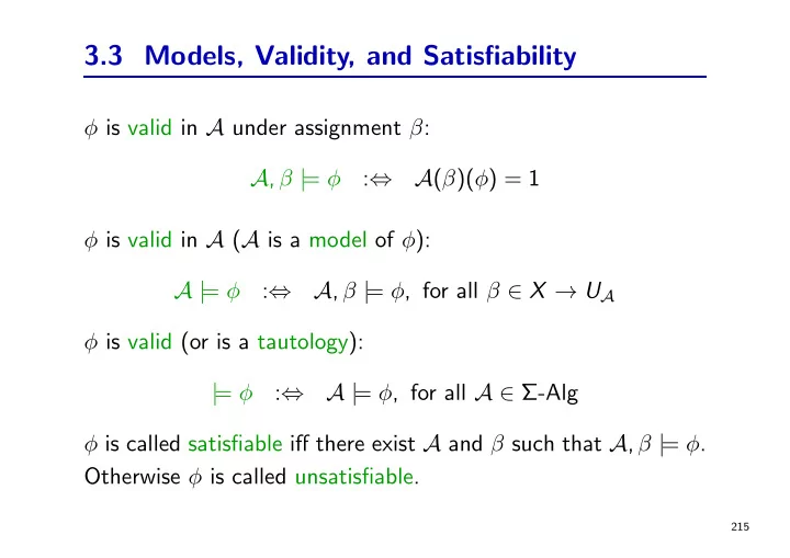
φ is valid in A under assignment β: A, β | = φ :⇔ A(β)(φ) = 1 φ is valid in A (A is a model of φ): A | = φ :⇔ A, β | = φ, for all β ∈ X → UA φ is valid (or is a tautology): | = φ :⇔ A | = φ, for all A ∈ Σ-Alg φ is called satisfiable iff there exist A and β such that A, β | = φ. Otherwise φ is called unsatisfiable.

215

Substitution Lemma

The following propositions, to be proved by structural induction, hold for all Σ-algebras A, assignments β, and substitutions σ. Lemma 3.3: For any Σ-term t A(β)(tσ) = A(β ◦ σ)(t), where β ◦ σ : X → A is the assignment β ◦ σ(x) = A(β)(xσ). Proposition 3.4: For any Σ-formula φ, A(β)(φσ) = A(β ◦ σ)(φ).

216

Substitution Lemma

Corollary 3.5: A, β | = φσ ⇔ A, β ◦ σ | = φ These theorems basically express that the syntactic concept

• f substitution corresponds to the semantic concept of an

assignment.

217

Entailment and Equivalence

φ entails (implies) ψ (or ψ is a consequence of φ), written φ | = ψ, if for all A ∈ Σ-Alg and β ∈ X → UA, whenever A, β | = φ, then A, β | = ψ. φ and ψ are called equivalent, written φ | = | ψ, if for all A ∈ Σ-Alg and β ∈ X → UA we have A, β | = φ ⇔ A, β | = ψ.

218

Entailment and Equivalence

Proposition 3.6: φ entails ψ iff (φ → ψ) is valid Proposition 3.7: φ and ψ are equivalent iff (φ ↔ ψ) is valid. Extension to sets of formulas N in the “natural way”, e. g., N | = φ :⇔ for all A ∈ Σ-Alg and β ∈ X → UA: if A, β | = ψ, for all ψ ∈ N, then A, β | = φ.

219

Validity vs. Unsatisfiability

Validity and unsatisfiability are just two sides of the same medal as explained by the following proposition. Proposition 3.8: Let φ and ψ be formulas, let N be a set of formulas. Then (i) φ is valid if and only if ¬φ is unsatisfiable. (ii) φ | = ψ if and only if φ ∧ ¬ψ is unsatisfiable. (iii) N | = ψ if and only if N ∪ {¬ψ} is unsatisfiable. Hence in order to design a theorem prover (validity checker) it is sufficient to design a checker for unsatisfiability.

220

Theory of a Structure

Let A ∈ Σ-Alg. The (first-order) theory of A is defined as Th(A) = { ψ ∈ FΣ(X) | A | = ψ } Problem of axiomatizability: For which structures A can one axiomatize Th(A), that is, can

• ne write down a formula φ (or a recursively enumerable set φ
• f formulas) such that

Th(A) = { ψ | φ | = ψ }? Analogously for sets of structures.

221

Two Interesting Theories

Let ΣPres = ({0/0, s/1, +/2}, ∅) and Z+ = (Z, 0, s, +) its standard interpretation on the integers. Th(Z+) is called Presburger arithmetic (M. Presburger, 1929). (There is no essential difference when one, instead of Z, considers the natural numbers N as standard interpretation.) Presburger arithmetic is decidable in 3EXPTIME (D. Oppen, JCSS, 16(3):323–332, 1978), and in 2EXPSPACE, using automata-theoretic methods (and there is a constant c ≥ 0 such that Th(Z+) ∈ NTIME(22cn)).

222

Two Interesting Theories

However, N∗ = (N, 0, s, +, ∗), the standard interpretation of ΣPA = ({0/0, s/1, +/2, ∗/2}, ∅), has as theory the so-called Peano arithmetic which is undecidable, not even recursively enumerable. Note: The choice of signature can make a big difference with regard to the computational complexity of theories.

223

3.4 Algorithmic Problems

Validity(φ): | = φ ? Satisfiability(φ): φ satisfiable? Entailment(φ,ψ): does φ entail ψ? Model(A,φ): A | = φ? Solve(A,φ): find an assignment β such that A, β | = φ. Solve(φ): find a substitution σ such that | = φσ. Abduce(φ): find ψ with “certain properties” such that ψ | = φ.

224

G¨

• del’s Famous Theorems
• 1. For most signatures Σ, validity is undecidable for Σ-formulas.

(Later by Turing: Encode Turing machines as Σ-formulas.)

• 2. For each signature Σ, the set of valid Σ-formulas is

recursively enumerable. (We will prove this by giving complete deduction systems.)

• 3. For Σ = ΣPA and N∗ = (N, 0, s, +, ∗), the theory Th(N∗) is

not recursively enumerable. These complexity results motivate the study of subclasses of formulas (fragments) of first-order logic Q: Can you think of any fragments of first-order logic for which validity is decidable?

225

Some Decidable Fragments

Some decidable fragments:

• Monadic class: no function symbols, all predicates unary;

validity is NEXPTIME-complete.

• Variable-free formulas without equality: satisfiability is

NP-complete. (why?)

• Variable-free Horn clauses (clauses with at most one positive

atom): entailment is decidable in linear time.

• Finite model checking is decidable in time polynomial in the

size of the structure and the formula.

226

Plan

Lift superposition from propositional logic to first-order logic.

227

3.5 Normal Forms and Skolemization

Study of normal forms motivated by

• reduction of logical concepts,
• efficient data structures for theorem proving,
• satisfiability preserving transformations (renaming),
• Skolem’s and Herbrand’s theorem.

The main problem in first-order logic is the treatment of

• quantifiers. The subsequent normal form transformations are

intended to eliminate many of them.

228

Prenex Normal Form (Traditional)

Prenex formulas have the form Q1x1 . . . Qnxn φ, where φ is quantifier-free and Qi ∈ {∀, ∃}; we call Q1x1 . . . Qnxn the quantifier prefix and φ the matrix of the formula.

229

Prenex Normal Form (Traditional)

Computing prenex normal form by the rewrite system ⇒P: (φ ↔ ψ) ⇒P (φ → ψ) ∧ (ψ → φ) ¬Qxφ ⇒P Qx¬φ (¬Q) ((Qxφ) ρ ψ) ⇒P Qy(φ{x → y} ρ ψ), ρ ∈ {∧, ∨} ((Qxφ) → ψ) ⇒P Qy(φ{x → y} → ψ), (φ ρ (Qxψ)) ⇒P Qy(φ ρ ψ{x → y}), ρ ∈ {∧, ∨, →} Here y is always assumed to be some fresh variable and Q denotes the quantifier dual to Q, i. e., ∀ = ∃ and ∃ = ∀.

230

Skolemization

Intuition: replacement of ∃y by a concrete choice function computing y from all the arguments y depends on. Transformation ⇒S (to be applied outermost, not in subformulas): ∀x1, . . . , xn∃y φ ⇒S ∀x1, . . . , xn φ{y → f (x1, . . . , xn)} where f /n is a new function symbol (Skolem function).

231

Skolemization

Together: φ ⇒∗

P

ψ

• prenex

⇒∗

S

χ

• prenex, no ∃

Theorem 3.9: Let φ, ψ, and χ as defined above and closed. Then (i) φ and ψ are equivalent. (ii) χ | = ψ but the converse is not true in general. (iii) ψ satisfiable (Σ-Alg) ⇔ χ satisfiable (Σ′-Alg) where Σ′ = (Ω ∪ SKF, Π), if Σ = (Ω, Π).

232

The Complete Picture

φ ⇒∗

P

Q1y1 . . . Qnyn ψ (ψ quantifier-free) ⇒∗

S

∀x1, . . . , xm χ (m ≤ n, χ quantifier-free) ⇒∗

OCNF

∀x1, . . . , xm

• leave out

k

• i=1

ni

• j=1

Lij clauses Ci

• φ′

N = {C1, . . . , Ck} is called the clausal (normal) form (CNF) of φ. Note: the variables in the clauses are implicitly universally quantified.

233

The Complete Picture

Theorem 3.10: Let φ be closed. Then φ′ | = φ. (The converse is not true in general.) Theorem 3.11: Let φ be closed. Then φ is satisfiable iff φ′ is satisfiable iff N is satisfiable

234

Optimization

The normal form algorithm described so far leaves lots of room for optimization. Note that we only can preserve satisfiability anyway due to Skolemization.

• size of the CNF is exponential when done naively; the

transformations we introduced already for propositional logic avoid this exponential growth;

• we want to preserve the original formula structure;
• we want small arity of Skolem functions (see next section).

235

3.6 Getting Small Skolem Functions

A clause set that is better suited for automated theorem proving can be obtained using the following steps:

• produce a negation normal form (NNF)
• apply miniscoping
• rename all variables
• skolemize

236

Negation Normal Form (NNF)

Apply the rewrite system ⇒NNF: φ[ψ1 ↔ ψ2]p ⇒NNF φ[(ψ1 → ψ2) ∧ (ψ2 → ψ1)]p if pol(φ, p) = 1 or pol(φ, p) = 0 φ[ψ1 ↔ ψ2]p ⇒NNF φ[(ψ1 ∧ ψ2) ∨ (¬ψ2 ∧ ¬ψ1)]p if pol(φ, p) = −1

237

Negation Normal Form (NNF)

¬Qx φ ⇒NNF Qx ¬φ ¬(φ ∨ ψ) ⇒NNF ¬φ ∧ ¬ψ ¬(φ ∧ ψ) ⇒NNF ¬φ ∨ ¬ψ φ → ψ ⇒NNF ¬φ ∨ ψ ¬¬φ ⇒NNF φ

238

Miniscoping

Apply the rewrite relation ⇒MS. For the rules below we assume that x occurs freely in ψ, χ, but x does not occur freely in φ: Qx (ψ ∧ φ) ⇒MS (Qx ψ) ∧ φ Qx (ψ ∨ φ) ⇒MS (Qx ψ) ∨ φ ∀x (ψ ∧ χ) ⇒MS (∀x ψ) ∧ (∀x χ) ∃x (ψ ∨ χ) ⇒MS (∃x ψ) ∨ (∃x χ)

239

Variable Renaming

Rename all variables in φ such that there are no two different positions p, q with φ|p = Qx ψ and φ|q = Q′x χ.

240

Standard Skolemization

Apply the rewrite rule: φ[∃x ψ]p ⇒SK φ[ψ{x → f (y1, . . . , yn)}]p where p has minimal length, {y1, . . . , yn} are the free variables in ∃x ψ, f /n is a new function symbol to φ

241