2 Preliminaries of the same size and covered by the same superset. - - PDF document

SLIDE 1

δ-Tolerance Closed Frequent Itemsets

James Cheng Yiping Ke Wilfred Ng Department of Computer Science and Engineering The Hong Kong University of Science and Technology {csjames, keyiping, wilfred}@cse.ust.hk Abstract

In this paper, we study an inherent problem of mining Frequent Itemsets (FIs): the number of FIs mined is often too large. The large number of FIs not only affects the min- ing performance, but also severely thwarts the application

• f FI mining. In the literature, Closed FIs (CFIs) and Max-

imal FIs (MFIs) are proposed as concise representations of

• FIs. However, the number of CFIs is still too large in many

cases, while MFIs lose information about the frequency of the FIs. To address this problem, we relax the restrictive definition of CFIs and propose the δ-Tolerance CFIs (δ- TCFIs). Mining δ-TCFIs recursively removes all subsets of a δ-TCFI that fall within a frequency distance bounded by δ. We propose two algorithms, CFI2TCFI and MineTCFI, to mine δ-TCFIs. CFI2TCFI achieves very high accuracy on the estimated frequency of the recovered FIs but is less effi- cient when the number of CFIs is large, since it is based on CFI mining. MineTCFI is significantly faster and consumes less memory than the algorithms of the state-of-the-art con- cise representations of FIs, while the accuracy of MineTCFI is only slightly lower than that of CFI2TCFI.

1 Introduction

Frequent Itemset (FI) mining [1, 2] is fundamental to many important data mining tasks such as associations [1], correlations [6], sequences [3], episodes [13], emerging pat- terns [8], indexing [17] and caching [18], etc. Over the last decade, a huge amount of research has been conducted on improving the efficiency of mining FIs and many fast algo- rithms [9] have been proposed. However, the mining oper- ation can easily return an explosive number of FIs, which not only severely thwarts the application of FIs, but also di- rectly affects the mining efficiency. To address this problem, Maximal Frequent Itemsets (MFIs) [4] and Closed Frequent Itemsets (CFIs) [14] are proposed as concise representations of FIs. MFIs are also FIs but none of their proper supersets is an FI. Since an FI of size n has (2n − 1) non-empty subset FIs, mining MFIs ef- fectively addresses the problem of too many FIs. However, most applications are not only interested in the patterns rep- resented by the FIs, but also require their occurrence fre- quency in the database for further analysis. For example, we need the frequency of the FIs to compute the support and confidence of association rules. MFIs, however, lose the frequency information of most FIs. On the contrary, the set of CFIs is a lossless representa- tion of FIs. CFIs are FIs that have no proper superset with the same frequency. Thus, we can retrieve the frequency

• f the non-closed FIs from their closed supersets. However,

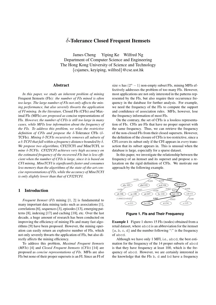
the definition of the closure of CFIs is too restrictive, since a CFI covers its subset only if the CFI appears in every trans- action that its subset appears in. This is unusual when the database is large, especially for a sparse dataset. In this paper, we investigate the relationship between the frequency of an itemset and its superset and propose a re- laxation on the rigid definition of CFIs. We motivate our approach by the following example.

abcd:100 abd:103 abc:103 acd:104 bcd:107 ab:106 ac:108 ad:107 bc:110 bd:130 cd:111 a:111 b:139 c:115 d:134

0.029 0.029 0.038 0.065 0.028 0.037 0.028 0.027 0.177 0.036 1-108/111=0.027 0.065 0.035 0.030

Figure 1. FIs and Their Frequency Example 1 Figure 1 shows 15 FIs (nodes) obtained from a retail dataset, where abcd is an abbreviation for the itemset {a, b, c, d} and the number following “:” is the frequency

• f abcd.

Although we have only 1 MFI, i.e., abcd, the best esti- mation for the frequency of the 14 proper subsets of abcd is that they have frequency at least 100, which is the fre- quency of abcd. However, we are certainly interested in the knowledge that the FIs b, d and bd have a frequency

SLIDE 2

significantly greater than that of other FIs. On the contrary, CFIs preserve the frequency information but all the 15 FIs are CFIs, even though the frequency of many FIs only differ slightly from that of their supersets. We investigate the relationship between the frequency of the FIs. In Figure 1, the number on each edge is computed as δ = (1 − frequency of Y

frequency of X ), where Y is X’s smallest su-

perset that has the greatest frequency. For CFIs, if we want to remove X from the mining result, δ has to be equal to 0, which is a restrictive condition in most cases. However, if we relax this equality condition to allow a small tolerance, say δ ≤ 0.04, we can immediately prune 11 FIs and retain

• nly abcd, bcd, bd and b (i.e., the bold nodes in Figure

1). The frequency of the pruned FIs can be accurately es- timated as the average frequency of the pruned FIs that are

• f the same size and covered by the same superset. For ex-

ample, ab, ac and ad are of the same size and covered by the same superset abcd; thus, their frequency is estimated as 106+108+107

3

= 107. ✷ We find that a majority of the FIs mined from most of the well-known real datasets [9], as well as from the preva- lently used synthetic datasets [12], exhibit the above char- acteristic in their frequency. Therefore, we propose to allow tolerance, bounded by a threshold δ, in the condition for the closure of CFIs, and define a new concise representation of FIs called the δ-Tolerance CFIs (δ-TCFIs). The notion of δ- tolerance greatly alleviates the restrictive definition of CFIs, as illustrated in the above example. We propose two algorithms to mine δ-TCFIs. Our algo- rithm, CFI2TCFI, is based on the fact that the set of CFIs is a lossless representation of FIs. CFI2TCFI first obtains the CFIs and then generates the δ-TCFIs by checking the condition of δ-tolerance on the CFIs. However, CFI2TCFI becomes inefficient when the number of CFIs is large. We study the closure of the δ-TCFIs and propose an-

• ther algorithm, MineTCFI, which makes use of the δ-

tolerance in the closure to perform greater pruning on the mining space. Since the pruning condition is a relaxation

• n the pruning condition of mining CFIs, MineTCFI is al-

ways more efficient than CFI2TCFI. The effectiveness of the pruning can also be inferred from Example 1 as the ma- jority of the itemsets can be pruned when the closure defin- ition of CFIs is relaxed. We compare our algorithms with FPclose [10], NDI [7], MinEx [5] and RPlocal [16], which are the state-of-the-art algorithms for mining the four respective concise represen- tations of FIs. Our experimental results on real datasets [9] show that the number of δ-TCFIs is many times (up to or- ders of magnitude) smaller than the number of itemsets ob- tained by the other algorithms. We also measure the error rate of the estimated frequency of the FIs that are recovered from the δ-TCFIs. In all cases, the error rate of CFI2TCFI is significantly lower than δ while that of MineTCFI is also considerably lower than δ. Most importantly, MineTCFI is significantly faster than all other algorithms, while the memory consumption of MineTCFI is also small and in most cases smaller than that of the other algorithms. Another important finding of mining δ-TCFIs is when δ increases, the error rate only increases at a much slower

• rate. Thus, we can further reduce the number of δ-TCFIs by

using a larger δ, while still attaining high accuracy.

• Organization. Section 2 gives the preliminaries. Then,

Section 3 defines the notion of δ-TCFIs and Section 4 presents the algorithms CFI2TCFI and MineTCFI. Section 5 reports the experimental results. Section 6 discusses re- lated work and Section 7 concludes the paper.

2 Preliminaries

Let I = {x1, x2, . . . , xN} be a set of items. An itemset (also called a pattern) is a subset of I. A transaction is an

• itemset. We say that a transaction Y supports an itemset X

if Y ⊇ X. For brevity, an itemset {xk1, xk2, . . . , xkm} is written as xk1xk2 . . . xkm in this paper. Let D be a database of transactions. The frequency of an itemset X, denoted as freq(X), is the number of transac- tions in D that support X. X is called a Frequent Itemset (FI) if freq(X) ≥ σ|D|, where σ (0 ≤ σ ≤ 1) is a user- specified minimum support threshold. X is called a Maxi- mal Frequent Itemset (MFI) if X is an FI and there exists no FI Y such that Y ⊃ X. X is called a Closed Frequent Itemset (CFI) if X is an FI and there exists no FI Y such that Y ⊃ X and freq(Y ) = freq(X).

3 δ-Tolerance Closed Frequent Itemsets

In this section, we first define the notion of δ-TCFIs. Then, we discuss how we estimate the frequency of the FIs that are recovered from the δ-TCFIs. Finally, we give an analysis on the error bound of the estimated frequency of the recovered FIs.

3.1 The Notion of δ-TCFIs

Definition 1 (δ-Tolerance Closed Frequent Itemset) An itemset X is a δ-tolerance closed frequent itemset (δ-TCFI) if and only if X is an FI and there exists no FI Y such that Y ⊃ X, |Y | = |X|+1, and freq(Y ) ≥ ((1 −δ)·freq(X)), where δ (0 ≤ δ ≤ 1) is a user-specified frequency toler- ance factor. We can define CFIs and MFIs by our δ-TCFIs as follows. Lemma 1 An itemset X is a CFI if and only if X is a 0- TCFI. Lemma 2 An itemset X is an MFI if and only if X is a 1-TCFI.

SLIDE 3

Corollary 1 The set of all CFIs and the set of all MFIs form the upper bound and the lower bound of the set of all δ-TCFIs, respectively. Example 2 Referring to the 15 FIs in Figure 1. Let δ = 0.04, then the set of 0.04-TCFIs is {b, bd, bcd, abcd}. For example, b is a 0.04-TCFI since b does not have a proper superset that has frequency greater than ((1 − 0.04) × 139) = 133. The FI a is not a 0.04-TCFI since (1 − freq(ac)

freq(a) ) = 0.027 < 0.04, and similarly for ac

since (1 − freq(acd)

freq(ac) ) = 0.037 < 0.04 and for acd since

(1 − freq(abcd)

freq(acd) ) = 0.038 < 0.04. Thus, they are recur-

sively covered by their superset that has 1 more item and then finally covered by the 0.04-TCFI abcd. The set of 0.07-TCFIs is {bd, abcd}, while the set of 1- TCFIs, i.e., MFIs, is {abcd}. However, the set of 0-TCFIs, i.e., CFIs, is all the 15 FIs. ✷ In the rest of the paper, we use F to denote the set of all FIs and T to denote the set of all δ-TCFIs, for a given δ.

3.2 Frequency Estimation

Given T , we can recover F (when demanded by appli- cations). The frequency of an FI X ∈ F can be estimated from the frequency of its supersets in T . We discuss the frequency estimation in this subsection. It is possible that for an FI X, there are more than one FI Y , where Y ⊃ X, |Y | = |X| + 1 and freq(Y ) ≥ ((1 − δ) · freq(X)). Among all these supersets of X, the one that has the greatest frequency can best estimate the frequency

• f X. Thus, we define this superset as the closest superset
• f X as follows.

Definition 2 (Closest Superset) Given an itemset X, let Y =

• Y : Y ⊃ X, |Y | = |X| + 1, and freq(Y ) =

MAX {freq(Y ′) : Y ′ ⊃ X, |Y ′| = |X| + 1}

• . Y is the

closest superset of X if Y ∈ Y and Y is lexicographically

• rdered before all other itemsets in Y.

Given an itemset X, we can follow a path of closest su- persets and finally reach one closest superset, which is a δ-

• TCFI. We define this δ-TCFI superset as the closest δ-TCFI

superset of X as follows. Definition 3 (Closest δ-TCFI Superset) Given n itemsets, X1, . . . , Xn, where for 1 ≤ i < n, Xi ⊂ Xi+1 and |Xi+1| = |Xi| + 1. Xn is the closest δ-TCFI superset of X1, if Xn ∈ T and for 1 ≤ i < n, Xi ∈ (F − T ) and Xi+1 is the closest superset of Xi. Example 3 Referring to Figure 1, the closest superset of a is ac, that of ac is acd and that of acd is abcd. For the two supersets of ab that have the same frequency, we choose abc as the closest superset of ab since abc is or- dered before abd. When δ = 0.04, abcd is the closest δ-TCFI superset of all its subsets that contain the item a, while bcd is the closest δ-TCFI superset of bc, cd and c. ✷ To estimate the frequency of the FIs with the same clos- est δ-TCFI superset Y , we group the FIs according to their size and define the frequency extension of Y as follows. Definition 4 (Frequency Extension) Given a δ-TCFI Y , let Xi = {X : |X| = |Y |−i and Y is the closest δ-TCFI super- set of X}, where 1 ≤ i ≤ m and m = MAX {i : Xi = ∅}. The frequency extension of Y , denoted as ext(Y ), is a list (ext(Y, 1), . . . , ext(Y, m)), where ext(Y, i), for 1 ≤ i ≤ m, is defined as ext(Y, i) =

• X∈Xi

freq(X) freq(Y )

|Xi| . The size of the frequency extension of Y , denoted as |ext(Y )|, is defined as |ext(Y )| = m. The frequency extension of Y is essentially a list of aver- aged frequency ratio grouped by the size of the FIs. With the frequency extension of Y , we can estimate the frequency of each X ∈ Xi, as (freq(Y ) · ext(Y, i)). We illustrate the frequency estimation by Example 4. Example 4 Referring to Example 3, let Y = abcd, then X1 = {abc, abd, acd}, X2 = {ab, ac, ad} and X3 = {a}. We have ext(abcd, 1) = ( 103

100 + 103 100 + 104 100)/3 =

1.03, ext(abcd, 2) = ( 106

100 + 108 100 + 107 100)/3 = 1.07 and

ext(abcd, 3) = 111

100/1 = 1.11.

Thus, the frequency of abc, abd and acd are estimated as (freq(abcd)·ext(abcd, 1)) = 103, the frequency of ab, ac and ad are estimated as (freq(abcd)·ext(abcd, 2)) = 107, while the frequency of a is estimated as (freq(abcd)· ext(abcd, 3)) = 111. ✷

3.3 Error Bound of Frequency Estimation

We now analyze the error bound of the frequency esti-

• mation. We first give Lemmas 3 and 4, which we use to

define the error bound. Lemma 3 ∀X ∈ (F − T ), ∃Y ∈ T such that Y ⊃ X and freq(Y ) ≥ ((1 − δ)|Y |−|X| · freq(X)). Lemma 4 For any δ-TCFI Y , 1 ≤ ext(Y, i) ≤

1 (1−δ)i .

Lemma 5 (Error Bound of Estimated Frequency) Given an FI X and X’s closest δ-TCFI superset Y , where |Y | − |X| = i. Let freq(X) be the exact frequency of X and

• freq(X) = (freq(Y )·ext(Y, i)) be the estimated frequency
• f X. Then,

φ − 1 ≤

g

freq(X) − freq(X) freq(X)

≤ 1 φ − 1, where φ = (1 − δ)i.

SLIDE 4

• Proof. Since

freq(X) = (freq(Y ) · ext(Y, i)), by Lemma 4, we have 0 ≤ freq(Y ) ≤ freq(X) ≤ freq(Y )

φ

. By Lemma 3, we have 0 ≤ freq(Y ) ≤ freq(X) ≤

freq(Y ) φ

. Thus, 0 ≤ (freq(Y )/ freq(Y )

φ

) ≤

g

freq(X) freq(X) ≤ ( freq(Y ) φ

/freq(Y )), i.e., φ ≤

g

freq(X) freq(X) ≤ 1 φ. Hence, (φ−1) ≤

g

freq(X)−freq(X) freq(X)

≤ ( 1

φ − 1).

✷ Lemma 5 gives the theoretical error bound of the fre- quency of an FI estimated from the frequency of its closest δ-TCFI superset. However, according to Definition 4, each ext(Y, i) of a δ-TCFI Y is taken as the average of the fre- quency ratio of the FIs in Xi over the frequency of Y , while the relative difference in the frequency of any two FIs in Xi is bounded by δ. Thus, in practice, the estimated frequency is highly accurate and the error bound is much smaller than the theoretical bound defined in Lemma 5, which is also verified by our extensive experiments.

4 Mining δ-TCFIs

In this section, we first present an algorithm that com- putes δ-TCFIs from the set of CFIs. Then, we propose a more efficient algorithm that employs pruning based on the closure of the δ-TCFIs.

4.1 Algorithm CFI2TCFI

Mining CFIs is in general much more efficient than min- ing FIs. Since the set of CFIs is a lossless representation of FIs, we devise an algorithm which takes advantage of the efficiency of mining CFIs. The algorithm first generates the CFIs and then computes the δ-TCFIs from the CFIs. Algorithm 1 CFI2TCFI

• 1. Mine the set of all CFIs;
• 2. Let Ci be the set of CFIs of size i;
• 3. for each i ≥ 1 do

4. for each X ∈ Ci do 5. Find X’s closest CFI superset, Y ; 6. if(∃Y s.t. freq(Y ) ≥ (1 − δ)|Y |−|X| · freq(X) ) 7. Update ext(Y ) with freq(X) and ext(X); 8. Delete X; 9. else 10. T ← T ∪ {X};

• 11. return T ;

Our algorithm, CFI2TCFI, is shown in Algorithm 1. We first generate all CFIs and partition them according to the size of the CFIs. Let Ci be the set of CFIs of size i. Starting from i = 1, we find the closest CFI superset of each CFI X (Line 5). Here, the closest CFI superset of X is defined as X’s CFI superset that has the smallest size and the greatest frequency among all other CFI supersets of X. If X’s clos- est CFI superset is not found, then X is a δ-TCFI and we include X in T (Line 10). If X has a closest CFI superset Y but freq(Y ) < ((1 − δ)|Y |−|X| · freq(X)), we also in- clude X in T (Line 10). Otherwise, we update ext(Y ) with freq(X) and ext(X), if any, and then delete X (Lines 7-8). CFI2TCFI computes the exact set of all δ-TCFIs and as we show in Section 5, the estimated frequency of the FIs re- covered from the δ-TCFIs obtained by CFI2TCFI is highly accurate in all cases. However, the search for the closest CFI superset of each CFI is costly when the number of CFIs is large. Thus, we propose a more scalable algorithm whose efficiency is not affected by the number of CFIs.

4.2 Algorithm MineTCFI

In this section, we discuss a very efficient algorithm, MineTCFI, for mining δ-TCFIs. We first describe the data structures used in MineTCFI in Sections 4.2.1 and 4.2.2. Then, we discuss an effective pruning in Section 4.2.3 and present the main algorithm in Section 4.2.4. 4.2.1 FP-Tree and FP-Growth The pattern-growth method, FP-growth, by Han et al. [11] is one of the most efficient methods for mining FIs, CFIs and MFIs [10]. We adopt the pattern-growth procedure as the skeleton of our algorithm MineTCFI. FP-growth mines FIs using an extended prefix-tree struc- ture called the FP-tree. As an example, Figure 2 shows the FP-tree, T∅, constructed from a database excerpt which gen- erates the FIs in Figure 1.

b: 139 root d: 4 c: 1 d: 130 c: 3 c: 4 a: 1 c: 107 a: 3 a: 3 a: 4 a: 100 item: freq head of node-links b: 139 d: 134 c: 115 a: 111 item label: freq Node v Header Table

Figure 2. The FP-Tree T∅ of Figure 1 FP-growth mines the set of FIs as follows. Given an FP- tree TX, where initially X = ∅ and T∅ is constructed from the original database. For each item x in TX.header, FP- growth follows the list of pointers to extract all paths from the root to the node representing x in TX. These paths form the conditional pattern base of Y = X ∪ {x}, denoted as BY , from which FP-growth constructs a local FP-tree, called the conditional FP-tree, denoted as TY . First, the frequent items in BY form TY .header. Then, FP-growth

SLIDE 5

re-orders the frequent items in each path in BY (the infre- quent items are discarded) and inserts the new path into TY . Figure 3 shows the conditional FP-tree, Tc, which is con- structed from the FP-tree T∅ in Figure 2.

root item: freq head of node-links d: 111 b: 110 Header Table d: 111 b: 107 b: 3

Figure 3. The Conditional FP-Tree Tc The above procedure is applied recursively until the con- ditional FP-tree consists of only a single path, P, from which FP-growth generates the itemsets represented by all sub-paths of P. 4.2.2 The δ-TCFI Tree A crucial operation in MineTCFI is the search for the su- persets of an itemset in the set of δ-TCFIs already discov-

• ered. Performing a subset testing by comparing the itemset

with every existing δ-TCFI is clearly inefficient. In mining CFIs, the subset testing can be efficiently processed by an FP-tree-like structure [10]. We thus develop a similar struc- ture, called the δ-TCFI tree, to be used for mining δ-TCFIs. To avoid testing all existing δ-TCFIs with X, a condi- tional δ-TCFI tree, CX, is created corresponding to the con- ditional FP-tree TX in each of the recursive pattern-growth procedure calls. Each CX is local since it contains only δ- TCFIs that are supersets of X. Thus, this local CX is much smaller than a global δ-TCFI tree that contains all δ-TCFIs. Each node v in CX has three fields: item label, level and δ-TCFI-link, where the item label indicates which item v represents, the level is the level of v in CX (the root is at Level 0), and the δ-TCFI-link is a pointer to the δ-TCFI represented by the root-to-v path. Since each δ-TCFI has a frequency extension, we keep the δ-TCFIs in an array so that the frequency extension will not be duplicated in each

• f the conditional δ-TCFI trees.

Like TX, CX also has a header table, denoted as CX.header. The items in CX.header are the same as the items in TX.header and in the same order. Each item x in CX.header is associate with an array, Ax. Each entry in Ax, Ax[l], is an array of pointers to all nodes in CX that have item label x and level l. Example 5 If δ = 0.027, we obtain seven δ-TCFIs after processing the item a. Figure 4 shows the global δ-TCFI tree, C∅, which contains the seven δ-TCFIs, and Figure 5(a) shows the conditional δ-TCFI tree, Cc, which contains only δ-TCFIs that are supersets of c. C∅ and Cc correspond to

c:3:abdc item: Aitem b: (1:v1) c: (1:v7),(2:v4,v6),(3:v3) item label:level:d-TCFI-link Node v Header Table d: (1:v5),(2:v2) d:2:abd c:2:abc c:2:adc b:1:ab d:1:ad c:1:ac root:0:Z v0 v1 v2 v4 v3 v5 v6 v7

• Figure 4. The Global δ-TCFI Tree C∅

item: Aitem d: (1:v2) Header Table b: (1:v1),(2:v3) d:1:acd v2 root:0:Z v0

• b:1:acb

v1 b:2:acdb v3 d:1:cdb v2 root:0:Z v0

• b:1:acb

b:2:cdb v3 v1 (a) Cc (Before Inserting cbd) (b) Cc (After Inserting cbd)

Figure 5. The Conditional δ-TCFI Tree Cc the FP-trees T∅ and Tc in Figures 2 and 3, respectively. Note that a is not in C∅.header and no node in C∅ represents a. This is because all δ-TCFIs containing a have already been generated and hence there is no need to include a in C∅. In C∅.header in Figure 4, “c: (1 : v7), (2 : v4, v6), (3 : v3)” means that Ac has three entries: Ac[1] has a pointer to v7 at Level 1, Ac[2] has pointers to v4 and v6 at Level 2, and Ac[3] has a pointer to v3 at Level 3. ✷ Update and Construction of δ-TCFI Tree. To insert a δ-TCFI Z = X ∪ Y into CX, we first sort the items in Y as the order of the items in CX.header. Then, the sorted Y is inserted into CX. If a prefix of the sorted Y already appears as a path in CX, we share the prefix but change the δ-TCFI- link, link, of each node on the path as follows. Assume link currently points to W, then link will point to Z if either (1) |Z| < |W| or (2) |Z| = |W| and freq(Z) > freq(W). If a new node is created for an item in Y , then its δ-TCFI-link points to Z. To construct a conditional δ-TCFI tree, CY , for an item x in CX.header, i.e., Y = X ∪ {x}, we first initialize CY .header based on the set of items in TY .header. Then, we access each node v in CX via its pointer in Ax and ex- tract the root-to-v path, P. After discarding the nodes on P that do not correspond to an item in CY .header, we re-order the remaining nodes on P according to CY .header and then insert the path into CY . The insertion is the same as the way we insert Z into CX that we just discussed above. Example 6 To insert the δ-TCFI cbd into Cc in Figure 5(a), we first sort bd as db according to Cc.header in Figure 5(a). Then, we share the path v2, v3. But the δ-TCFI- link of v2 and v3 will be changed to point to cdb, since freq(cdb) > freq(acd) and |cdb| < |acdb|. The δ-

SLIDE 6

TCFI tree after the insertion of cbd is shown in Figure 5(b), where Cc.header remains unchanged as in Figure 5(a). ✷ 4.2.3 Closure-Based Pruning The efficiency of CFI mining is mainly due to the pruning based on the closure of CFIs. We make use of the tolerance in the closure of the δ-TCFIs to achieve greater pruning in MineTCFI. The pruning is described as follows. Given an FI X and X’s conditional FP-tree TX. Let Y = X ∪ {x}, where x is an item in TX.header, and F(TY ) be the set of FIs to be generated from Y ’s conditional FP-tree TY . We say that Y is covered if there exists a δ-TCFI Z such that Z ⊃ Y and freq(Z) ≥ ((1 − δ)|Z|−|Y | · freq(Y )). At the time when we generate Y , if Y is already covered, then we prune all FIs in F(TY ) and thus TY will not be constructed. The above pruning can be directly applied to mine 0- TCFIs (i.e., CFIs), since the FIs in F(TY ) must already be covered by some 0-TCFIs that are found before we generate Y . However, when δ > 0, a minority of FIs in F(TY ) may not be covered by any existing δ-TCFI due to the frequency tolerance in the closure. Some of this minority of FIs may later become δ-TCFIs. However, only a very small number

• f these FIs will become δ-TCFIs. Missing these δ-TCFIs

will only slightly degrade the accuracy of the estimated fre- quency of the recovered FIs, while we can still recover all FIs from their other δ-TCFI supersets. But to improve the accuracy of the estimated frequency, we apply an additional checking to prevent pruning these potential δ-TCFIs, as de- scribed by the following heuristic. Heuristic 1 Let H be the set of frequent items in Y ’s condi- tional pattern base, BY , and Y ′ = Y ∪ H. If Y is covered and Y ′ is also covered, then we prune all FIs in F(TY ). Heuristic 1 is based on the proximity of frequency of the itemsets found in most datasets: if Y is covered and Y ′, which is the largest possible superset of Y that can be generated from TY , is also covered, then most likely other FIs in-between Y and Y ′ are also covered. However, at the time when we generate Y , the frequency

• f Y ′ has not been determined and hence we cannot check

the condition whether Y ′ is covered. However, we find that if there exists a δ-TCFI, Z′, which is a superset of Y ′, then in most cases Y ′ is covered (due to the proximity of fre- quency). Thus, we obtain the following heuristic. Heuristic 2 If Y is covered and there exists a δ-TCFI, Z′, such that Z′ ⊃ Y ′, then we prune all FIs in F(TY ). Heuristic 2 implies that we only need to check the subset- superset condition without knowing the frequency of Y ′. To further increase the probability that other FIs in F(TY ) are also covered, we can add one more level of checking that |ext(Z′)| ≥ (|Z′| − |Y | − 1), which means that Z′ has already covered subsets of size from (|Y |+1) to (|Z′|−1). Let U and V be any two such subsets covered by Z′, where |V | = |U| + 1, then the difference between the frequency

• f U and that of V is bounded by δ. Since the FIs in F(TY )

also share the same superset Z′, this proximity of frequency

• f other subsets of Z′ implies a high probability that the FIs

in F(TY ) are also covered. Thus, we obtain Heuristic 3. We first define that Y ′ is conditionally covered by a δ- TCFI Z′ if Z′ ⊃ Y ′ and |ext(Z′)| ≥ (|Z′| − |Y | − 1). Heuristic 3 If Y is covered and there exists a δ-TCFI, Z′, such that Y ′ is conditionally covered by Z′, then we prune all FIs in F(TY ). Example 7 Based on T∅ in Figure 2, if δ=0.07, we first find abdc is a 0.07-TCFI after processing a. Then, when we process c in T∅.header, there are two frequent items {d, b} in Bc, from which we can generate cb, cbd and

• cd. Since c is covered by abdc, (c ∪ {d, b}) ⊂ abdc

and |ext(abdc)| = 3 > (|abdc| − |c| − 1) = 2, we can be sure that the frequency of cb, cbd and cd can be estimated with ext(abdc). Thus, we can prune cb, cbd and cd. Note that if δ=0.04, then abdc does not cover c. Hence, we will continue from c and find the δ-TCFI cbd. ✷ Coverage Testing. We now discuss how Heuristic 3 can be efficiently processed using the δ-TCFI tree. Given an FI X and X’s δ-TCFI tree CX, let Y = X ∪ {x}, where x is an item in CX.header. We find the superset

• f Y in CX as follows. We access Ax in CX.header and

follow the pointers in Ax[i] (i ≥ 1, starting from i = 1) to visit the nodes that have item label x and are at Level i

• f CX. For each node v visited, let v’s δ-TCFI-link point

to Z, we check if Y is covered by Z by testing freq(Z) ≥ ((1 − δ)|Z|−|Y | · freq(Y )). If Y is covered by Z, then Heuristic 3 requires us to check if Y ′ = Y ∪ H is conditionally covered, where H is the set of frequent items in BY . To check this, we first sort the items in H as their order in CX.header. Let the sorted H be H = x1x2 · · · xk. We access Axk of the item xk in CX.header. We first process Axk [k], which contains the pointers to the nodes at Level k in CX. For each node v accessed via a pointer in Axk [k], we check if the root-to-v path represents a superset of H. The checking starts from v’s parent up to the root and we compare both the item label and the level

• f each node along the path. When we compare xi (1 ≤

i ≤ k − 1) with a node u, if u’s level is smaller than i, we stop the comparison and move on to process the next node pointer in Axk [k], and then the pointers in Axk [k +1] when we finish Axk [k] and so on. Since CX is a local δ-TCFI tree containing only δ-TCFIs that are supersets of X, the number of comparisons is usu- ally small. In addition, those δ-TCFIs that are accessed via

SLIDE 7

pointers in Axk [i] (∀i < k) are not compared, since the paths from the root to those nodes have less nodes than the number of items in H and hence cannot be supersets of H. In the same way, the level of a node also helps terminate many of the subset testings earlier. When a root-to-v path is found to be a superset of H, let v’s δ-TCFI-link point to Z′, we check if Y ′ is conditionally covered by Z′ by testing |ext(Z′)| ≥ (|Z′|−|Y |−1). If Y ′ is conditionally covered by Z′, Heuristic 3 is then applied and all FIs in F(TY ) are pruned. In MineTCFI, if Y is covered by Z and Y ′ is condition- ally covered (by Z′), we need to determine if Z is the closest δ-TCFI superset of Y in order to update the frequency ex- tension of Z. To do this, we need to check whether the size

• f Z is the smallest among all δ-TCFIs that are supersets
• f Y . But this does not mean that we need to process all

δ-TCFIs that are supersets of Y . We do not process any of the δ-TCFIs that are accessed via the pointers in Ax[j], ∀j > |Z|−|X|, because the pointers in Ax[j] link to δ-TCFIs

• f size at least (|X| + j) > |Z|. In most cases, Y ’s closest

δ-TCFI superset is found via a pointer in Ax[1] and rarely do we go through many entries of Ax. 4.2.4 Algorithm MineTCFI We now present our algorithm, MineTCFI, as shown in Algorithm 2. After constructing the global FP-tree T∅, MineTCFI invokes the recursive pattern-growth procedure GenTCFI, which is shown in Procedure 1. In Procedure 1, the processing of IsCovered (Lines 4 and 14), IsCondCovered (Line 15) and the search for the closest δ-TCFI superset (Lines 5 and 16) are discussed in Coverage Testing in Section 4.2.3. Procedure 1 can be divided into two parts: when the input conditional FP-tree, TX, consists

• f only one single path (Lines 1-9), and when TX has more

than one path (Lines 10-23). When TX consists of only one single path P, GenTCFI generates all itemsets which satisfy locally the condition of a δ-TCFI. Then, for each local δ-TCFI Y , GenTCFI checks if Y is covered. If Y is not covered, then Y is a δ-TCFI and we add it to T (Line 8). GenTCFI also inserts Y into all the conditional δ-TCFI trees which are constructed along the path of the previous recursive calls of GenTCFI (Line 9), so that the future recursive calls can construct their conditional δ-TCFI trees correctly. If Y is covered, GenTCFI finds Y ’s closest δ-TCFI superset Z from CX and updates Z’s fre- quency extension with the frequency of Y (Lines 5-6). When TX consists of more than one path, GenTCFI processes each item x in TX.header as follows. First, GenTCFI constructs the conditional pattern base BY of Y = X ∪ {x}. Let H be the set of frequent items in BY . If Y is covered and (Y ∪ H) is conditionally covered, by Heuristic 3, GenTCFI prunes all supersets of Y that are to Algorithm 2 MineTCFI

• 1. Construct the global FP-tree, T∅;
• 2. Initialize the global δ-TCFI tree, C∅;
• 3. T ← ∅;
• 4. Invoke GenTCFI(T∅, C∅, T );
• 5. Return T ;

Procedure 1 GenTCFI(TX, CX, T )

• 1. if(TX is a single path, P)

2. Generate all local δ-TCFIs from P; 3. for each local δ-TCFI, Y , generated do 4. if( IsCovered(Y, CX) = true ) 5. Find Y ’s closest δ-TCFI superset, Z; 6. Update ext(Z) with freq(Y ); 7. else 8. T ← T ∪ {Y }; 9. Insert Y into all CX’s predecessor δ-TCFI trees in the recursive-call stack;

• 10. else

11. for each x in TX.header do 12. Y ← X ∪ {x}; 13. Let H be the set of frequent items in BY ; 14. if( IsCovered(Y, CX) = true ) 15. if( IsCondCovered(Y ∪ H, CX) = true ) /∗ Prune all supersets of Y ∗/ 16. Find Y ’s closest δ-TCFI superset, Z; 17. Update ext(Z) with freq(Y ); 18. else 19. Construct Y ’s conditional FP-tree, TY , and Y ’s conditional δ-TCFI tree, CY ; 20. GenTCFI(TY , CY , T ); 21. else /∗ IsCovered(Y, CX) = false ∗/ 22. Construct Y ’s conditional FP-tree, TY , and Y ’s conditional δ-TCFI tree, CY ; 23. GenTCFI(TY , CY , T );

be generated from TY (Lines 14-17). Otherwise, GenTCFI constructs Y ’s conditional FP-tree TY and conditional δ- TCFI tree CY (Lines 19 and 22). The recursive procedure is then called to process on TY and CY (Lines 20 and 23).

5 Experimental Results

We now evaluate our approach of mining δ-TCFIs. We run all experiments on a PC with an Intel P4 3.2GHz CPU and 2GB RAM, running Linux 64-bit. Datasets. We use the real datasets from the popular FIMI Dataset Repository [9]. We choose three datasets with the following representative characteristics. For a wide range

• f values of σ:
• pumsb*: the number of CFIs is orders of magnitude

smaller than that of FIs, but is orders of magnitude larger than that of MFIs.

SLIDE 8

• accidents: the number of CFIs is almost the same

as that of FIs, and is orders of magnitude larger than that of MFIs.

• mushroom: the number of CFIs is orders of magni-

tude smaller than that of FIs, but is only a few times larger than that of MFIs. Algorithms for Comparison. We compare our algorithms CFI2TCFI and MineTCFI with the following algorithms:

• FPclose [10]: the winner of FIMI 2003 [9] and one of

the fastest public implementations for mining CFIs.

• NDI [7]: the algorithm (the faster DFS approach) for

computing the set of non-derivable FIs (NDIs).

• MinEx [5]: the algorithm for mining the set of frequent

δ-free-sets.

• RPlocal [16]: the faster algorithm (than RPglobal)

for computing the representative patterns of the δ- clusters.

5.1 Performance at Different Minimum Support Thresholds

We first study the performance of the different algo- rithms by varying the minimum support threshold σ. We fix δ=0.05 for both pumsb* and accidents. For mushroom, since the difference between the number of CFIs and that of MFIs is much smaller than the other two datasets, we set a larger δ = 0.2 to obtain a greater reduc- tion for the algorithms with the parameter δ. We use the same δ for CFI2TCFI, MineTCFI and RPlo-

• cal. However, the δ defined in MinEx is an absolute value.

Thus, in each case we compare with MinEx, we find a δ for MinEx such that the error rate of MinEx approximately matches that of MineTCFI. 5.1.1 Number of Itemsets and Error Rate We compare the size of each of the concise representations

• f FIs. For simplicity, we use Num(alg) to denote the num-

ber of itemsets obtained by the algorithm alg. Figures 6 to 8 report the number of itemsets returned by each algorithm. In most cases, Num(CFI2TCFI) and Num(MineTCFI) are about an order of magnitude smaller than Num(FPclose) and Num(NDI), many times smaller than Num(MinEx), and on average 2 times smaller than Num(FPclose). In all cases, the number of δ-TCFIs ob- tained by both MineTCFI and CFI2TCFI is very close to the number of MFIs. Table 1 shows the error rate of the estimated frequency

• f the FIs recovered from the δ-TCFIs. We can see the er-

ror rate of CFI2TCFI is much lower than δ in all cases. The error rate of MineTCFI is higher but still lower than δ, espe- cially that for mushroom is only 1/10 of δ. The error rate

0.1 0.2 0.3 0.4 0.5 10

1

10

2

10

3

10

4

10

5

10

6

Minimum Support Threshold σ Number of Itemsets

FPclose NDI MinEx RPlocal MineTCFI CFI2TCFI MFI

Figure 6. Number of Itemsets (pumsb*)

0.1 0.2 0.3 0.4 0.5 10

2

10

3

10

4

10

5

10

6

10

7

Minimum Support Threshold σ Number of Itemsets

FPclose NDI MinEx RPlocal MineTCFI CFI2TCFI MFI

Figure 7. Number of Itemsets (accidents)

0.01 0.02 0.03 0.04 0.05 10

3

10

4

10

5

Minimum Support Threshold σ Number of Itemsets

FPclose NDI MinEx RPlocal MineTCFI CFI2TCFI MFI

Figure 8. Number of Itemsets (mushroom)

• f MineTCFI is higher than CFI2TCFI because MineTCFI

is only able to include partially the frequency of the subsets

• f a δ-TCFI in its frequency extension, as some of the sub-

sets are pruned. The error rate of MinEx is the same as that

• f MineTCFI. NDIs and CFIs are lossless representations
• f FIs, while the error rate of RPlocal is bounded by δ.

pumsb* accidents mushroom (δ = 0.05) (δ = 0.05) (δ = 0.2) CFI2TCFI 0.01 0.01 0.01 MineTCFI 0.03 0.04 0.02

Table 1. Error Rate of Estimated Frequency 5.1.2 Running Time and Memory Consumption Figure 9 reports the running time and memory consumption

• f the algorithms. We truncate the time and memory that are
• rders of magnitude larger than the largest points presented

SLIDE 9

0.1 0.2 0.3 0.4 0.5 20 40 60 80 Minimum Support Threshold σ Running Time (sec) FPclose NDI RPlocal MineTCFI CFI2TCFI

(a1) Running Time (pumsb*)

0.1 0.2 0.3 0.4 0.5 20 40 60 80 100 Minimum Support Threshold σ Memory Consumption (MB) FPclose NDI RPlocal MineTCFI CFI2TCFI

(a2) Memory Usage (pumsb*)

0.1 0.2 0.3 0.4 0.5 50 100 150 200 250 300 Minimum Support Threshold σ Running Time (sec) FPclose NDI RPlocal MineTCFI CFI2TCFI

(b1) Running Time (accidents)

0.1 0.2 0.3 0.4 0.5 50 100 150 200 Minimum Support Threshold σ Memory Consumption (MB) FPclose NDI RPlocal MineTCFI CFI2TCFI

(b2) Memory Usage (accidents)

0.01 0.02 0.03 0.04 0.05 5 10 15 20 Minimum Support Threshold σ Running Time (sec) FPclose NDI RPlocal MineTCFI CFI2TCFI

(c1) Running Time (mushroom)

0.01 0.02 0.03 0.04 0.05 5 10 15 20 25 30 Minimum Support Threshold σ Memory Consumption (MB) FPclose NDI RPlocal MineTCFI CFI2TCFI

(c2) Memory Usage (mushroom)

Figure 9. Time and Memory for Varying σ in the respective figures, since most of the time and memory usage are small and will be squeezed into a single line if we use a logarithmic scale. It is obvious from Figures 9 (a1), (b1) and (c1) that MineTCFI, which is the lowest line in all figures, is sig- nificantly faster than all other algorithms. The running time

• f RPlocal is the closest to that of MineTCFI but still about

3 times longer on average. CFI2TCFI is also fast in most of the cases, except when the number of CFIs is large. The memory consumption of the algorithms is small in most cases, except that CFI2TCFI and FPclose use more memory when the number of CFIs is large. For mushroom as shown in Figure 9 (c2), MineTCFI consumes more mem-

• ry than other algorithms but the difference is only 2MB.

However, in most of the other cases, MineTCFI has the low- est memory consumption among all algorithms, as shown in Figures 9 (a2) and (b2).

5.2 Effect of Different Values of δ

We now study the effect of different values of δ on min- ing δ-TCFIs. We test on the two larger datasets pumsb* and accidents. We fix σ at 0.3 and vary δ from 0.001 (a sufficiently low error rate in our opinion) to 0.2 (a δ at which the set of δ-TCFIs is almost the set of MFIs).

0.001 0.01 0.05 0.1 0.15 0.2 10

2

10

3

10

4

10

5

Frequency Tolerance Factor δ Number of Itemsets FPclose MineTCFI CFI2TCFI MFI

(a) No. of Itemsets (pumsb*)

0.001 0.01 0.05 0.1 0.15 0.2 10

3

10

4

10

5

10

6

Frequency Tolerance Factor δ Number of Itemsets FPclose MineTCFI CFI2TCFI MFI

(b) No. of Itemsets (accidents)

Figure 10. Different Values of δ Figures 10 (a) and (b) show the number of δ-TCFIs ob- tained by CFI2TCFI and MineTCFI, as well as the number

• f CFIs and MFIs as references. The number of δ-TCFIs is

about 4 to 5 times smaller than that of CFIs at δ = 0.001 and already becomes over an order of magnitude smaller at δ = 0.01. The number of δ-TCFIs is within 2 times of that

• f MFIs at δ = 0.05 and is almost the same as that of MFIs

at δ = 0.2.

0.001 0.01 0.05 0.1 0.15 0.2 10

−5

10

−4

10

−3

10

−2

10

−1

Frequency Tolerance Factor δ Error Rate MineTCFI (accidents) MineTCFI (pumsb*) CFI2TCFI (accidents) CFI2TCFI (pumsb*)

Figure 11. Error Rate of Different δ Figure 11 shows the error rate of CFI2TCFI and MineTCFI for pumsb* and accidents. At δ = 0.001, the error rate of CFI2TCFI and MineTCFI is significantly (up to 20 times) smaller than δ, except that of MineTCFI for pumsb* which is approximately 0.001. The error rate increases only slightly for large values of δ. For pumsb* at 0.05 ≤ δ ≤ 0.2 and accidents at 0.1 ≤ δ ≤ 0.2, the error rate increases only within the range of 0.01. This result shows that the actual error rate does not grow with the theoretical error bound given in Lemma 5, but re- mains to be small when δ becomes large. This is an impor- tant finding since for many applications the user is allowed to specify a large δ, while we can still achieve high accu- racy, which is not largely affected by δ, and obtain a very concise set of δ-TCFIs. The small error rate also demon-

SLIDE 10

strates the need for the frequency extension of a δ-TCFI in maintaining high accuracy of the estimated frequency.

6 Related Work

In addition to MFIs [4] and CFIs [14] we have discussed in Section 1, we are aware of the work by Xin et al. [16] which uses a similar notion of closeness measure of fre- quency by δ. They define a set of itemsets, S, to form a cluster if ∃Y (called a representative pattern), such that ∀X ∈ S, X ⊆ Y and (1 − freq(Y )

freq(X)) ≤ δ.

However, this definition is non-recursive, while the definition of our δ-TCFIs removes the redundant subsets recursively. Thus,

• ur approach is able to achieve better compression as evi-

denced by experimental results. We note that the number of δ-TCFIs can be significantly reduced when a relaxed mini- mum support threshold is used as in [16]. However, in our experiments, we do not relax the minimum support thresh-

• ld for both RPlocal and our algorithms, as to be fair to
• ther algorithms under comparison.

Boulicaut et al. [5] define an itemset X as a δ-free-set if ∀X′ ⊆ X, ∄Y ⊂X′ such that (freq(Y )−freq(X′))≤δ. The frequency of an FI X is estimated from its subsets; thus, an extra set of border itemsets is required in order to de- termine whether X is frequent. Calders and Goethals [7] utilize the inclusion-exclusion principle to deduce the lower bound and the upper bound for the frequency of an itemset and define an itemset as non-derivable if the lower bound and the upper bound are not equal. The set of NDIs is a lossless representation of FIs but can be still too large in some cases. Pei et al. [15] propose two types of condensed FI bases to approximate the frequency of itemsets with a user-defined error bound k. The frequency of an FI can be derived from either its subsets or supersets in the FI base.

7 Conclusions

We propose δ-TCFIs as a concise and flexible represen- tation of FIs. The notion of δ-tolerance allows us to flexibly tune δ to enjoy the benefits of both MFIs and CFIs: we can prune a great amount of redundant patterns from the min- ing result as do MFIs, while we can retain the frequency information of the recovered FIs as do CFIs. Experimental results verify that in all cases, the number of δ-TCFIs is very close to the number of MFIs and much smaller than all other existing concise representations of FIs [10, 7, 5, 16]. The results also show that the actual error rate of the estimated frequency of the recovered FIs is much lower than the theo- retical error bound. In particular, our algorithm CFI2TCFI attains an error rate significantly lower than δ in all cases. CFI2TCFI is also shown to be very efficient in most cases except when the number of CFIs is large. Our second algo- rithm MineTCFI attains an accuracy slightly lower than that

• f CFI2TCFI; however, MineTCFI is significantly faster

than all other algorithms [10, 7, 5, 16] in all cases and also consumes less memory in most cases. Acknowledgement. This work is partially supported by RGC CERG under grant number HKUST6185/03E. The authors would like to thank Prof. G¨

• sta Grahne for pro-

viding us FPclose, Dr. Bart Goethals for providing us NDI,

• Prof. Christophe Rigotti for providing us MinEx, and Prof.

Jiawei Han and Mr. Dong Xin for providing us RPlocal.

References

[1] R. Agrawal, T. Imielinski, and A. N. Swami. Mining Asso- ciation Rules between Sets of Items in Large Databases. In

• Proc. of SIGMOD, 1993.

[2] R. Agrawal and R. Srikant. Fast Algorithms for Mining As- sociation Rules. In Proc. of VLDB, 1994. [3] R. Agrawal and R. Srikant. Mining Sequential Patterns. In

• Proc. of ICDE, 1995.

[4] R. Bayardo. Efficiently Mining Long Patterns from Data-

• bases. In Proc. of SIGMOD, 1998.

[5] J.F. Boulicaut, A. Bykowski and C. Rigotti. Free-Sets: a Condensed Representation of Boolean Data for the Approx- imation of Frequency Queries. In DMKD 7(1):5-22, 2003. [6] S. Brin, R. Motwani, and C. Silverstein. Beyond Market Basket: Generalizing Association Rules to Correlations. In

• Proc. of SIGMOD, 1997.

[7] T. Calders and B. Goethals. Mining All Non-derivable Fre- quent Itemsets. In Proc. of PKDD, 2002. [8] G. Dong and J. Li. Efficient Mining of Emerging Patterns: Discovering Trends and Differences. In Proc. of KDD, 1999. [9] B. Goethals and M. Zaki. FIMI 2003 workshop. In Proc. of the ICDM Workshop on Frequent Itemset Mining Implemen- tations, 2003. [10] G. Grahne and J. Zhu. Efficiently Using Prefix-trees in Min- ing Frequent Itemsets. In IEEE ICDM Workshop on Fre- quent Itemset Mining Implementations (FIMI 03), 2003. [11] J. Han, J. Pei, and Y. Yin. Mining Frequent Patterns without Candidate Generation. In Proc. of SIGMOD, 2000. [12] IBM Quest Data Mining Project. The Quest re- tail transaction data generator. http://www. almaden.ibm.com/software/quest/, 1996. [13] H. Mannila, H. Toivonen, and A. I. Verkamo. Discovery of Frequent Episodes in Event Sequences. In DMKD, 1:259- 289, 1997. [14] N. Pasquier, Y. Bastide, R. Taouil, and L. Lakhal. Discover- ing Frequent Closed Itemsets for Association Rules. In Proc.

• f ICDT, 1999.

[15] J. Pei, G. Dong, W. Zou, and J. Han. Mining Condensed Frequent-Pattern Bases. In Knowl. Inf. Syst. 6(5): 570-594, 2004. [16] D. Xin, J. Han, X. Yan, and H. Cheng. Mining Compressed Frequent-Pattern Sets. In Proc. of VLDB, 2005. [17] X. Yan, P. Yu, and J. Han. Graph Indexing: A frequent Structure-Based Approach. In Proc. of SIGMOD, 2004. [18] L. H. Yang, M. L. Lee, W. Hsu. Efficient Mining of XML Query Patterns for Caching. In Proc. of VLDB, 2003.