18.05 Exam 2 review problems with solutions Spring 2014 Jeremy Orloff - PDF document

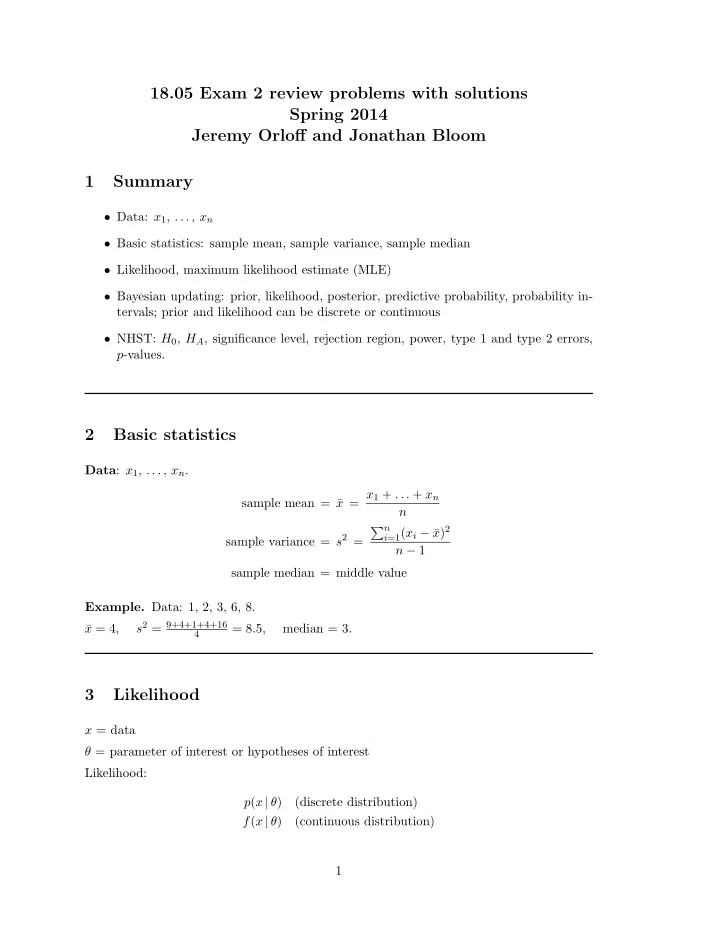
18.05 Exam 2 review problems with solutions Spring 2014 Jeremy Orloff and Jonathan Bloom 1 Summary • Data: x 1 , . . . , x n • Basic statistics: sample mean, sample variance, sample median • Likelihood, maximum likelihood estimate (MLE) • Bayesian updating: prior, likelihood, posterior, predictive probability, probability in- tervals; prior and likelihood can be discrete or continuous • NHST: H 0 , H A , significance level, rejection region, power, type 1 and type 2 errors, p ­values. 2 Basic statistics Data : x 1 , . . . , x n . x 1 + . . . + x n sample mean = x ¯ = n n ( x i − x ¯) 2 2 i =1 sample variance = s = n − 1 sample median = middle value Example. Data: 1, 2, 3, 6, 8. 2 9+4+1+4+16 x ¯ = 4, s = = 8 . 5, median = 3. 4 3 Likelihood x = data θ = parameter of interest or hypotheses of interest Likelihood: p ( x | θ ) (discrete distribution) f ( x | θ ) (continuous distribution) 1

2 18.05 Exam 2 review problems with solutions Log likelihood : ln( p ( x | θ )) . ln( f ( x | θ )) . Likelihood examples. Find the likelihood function of each of the following. 1. Coin with probability of heads θ . Toss 10 times get 3 heads. 2. Wait time follows exp( λ ). In 5 independent trials wait 3,5,4,5,2 3. Usual 5 dice. Two independent rolls, 9, 5. (Likelihood given in a table) 4. Independent x 1 , . . . , x n ∼ N( µ, σ 2 ) 5. x = 6 drawn from uniform(0 , θ ) 6. x ∼ uniform(0 , θ ) Solutions. 10 θ 3 (1 − θ ) 7 . 1. Let x be the number of heads in 10 tosses. P ( x = 3 | θ ) = 3 2. f (data | λ ) = λ 5 e − λ (3+5+4+5+2) = λ 5 e − 19 λ 3. Hypothesis θ Likelihood P (data | θ ) 4­sided 0 6­sided 0 8­sided 0 12­sided 1/144 20­sided 1/400 − [ ( x 1 − µ )2+( x 2 − µ )2+ ... +( xn − µ )2 ] n � � √ 1 4. f (data | µ, σ ) = e 2 σ 2 2 πσ � 0 if θ < 6 5. f ( x = 6 | θ ) = 1 /θ if 6 ≤ θ � 0 if θ < x or x < 0 6. f ( x | θ ) = 1 /θ if 0 ≤ x ≤ θ 3.1 Maximum likelihood estimates (MLE) Methods for finding the maximum likelihood estimate (MLE). • Discrete hypotheses: compute each likelihood • Discrete hypotheses: maximum is obvious • Continuous parameter: compute derivative (often use log likelihood) • Continuous parameter: maximum is obvious Examples. Find the MLE for each of the examples in the previous section.

3 18.05 Exam 2 review problems with solutions Solutions. 10 1. ln( f ( x − 3 | θ ) = ln + 3 ln( θ ) − 7 ln(1 − θ ). 3 3 7 3 ˆ Take the derivative and set to 0: + = 0 ⇒ θ = . θ 1 − θ 10 2. ln( f (data | λ ) = 5 ln( λ ) − 19 λ . 5 5 ˆ Take the derivative and set to 0: − 19 = 0 ⇒ λ = . λ 19 3. Read directly from the table: MLE = 12­sided die. 4. For the exam do not focus on the calculation here. You should understand the idea that we need to set the partial derivatives with respect to µ and σ to 0 and solve for the critical ˆ 2 ). point (ˆ µ, σ ˆ) 2 ˆ ( x i − µ µ = x , σ 2 = The result is ˆ . n 5. Because of the term 1 /θ in the likelihood, the likelihood is at a maximum when θ is as ˆ small as possible. answer: : θ = 6. ˆ = x . 6. This is identical to problem 5 except the exact value of x is not given. answer: θ 4 Bayesian updating 4.1 Bayesian updating: discrete prior-discrete likelihood. Jon has 1 four­side, 2 six­sided, 2 eight­sided, 2 twelve sided, and 1 twenty­sided dice. He picks one at random and rolls a 7. 1. For each type of die, find the posterior probability Jon chose that type. 2. What are the posterior odds Jon chose the 20­sided die? 3. Compute the prior predictive probability of rolling a 7 on the first roll. 4. Compute the posterior predictive probability of rolling an 8 on the second roll. Solutions. 1. . Make a table. (We include columns to answer question 4.) Hypothesis Prior Likelihood Unnorm. posterior posterior likelihood unnorm. posterior θ P ( θ ) f ( x 1 = 7 | θ ) f ( θ | x 1 = 7) P ( x 2 = 8 | θ ) 4­sided 1/8 0 0 0 0 0 6­sided 1/4 0 0 0 0 0 8­sided 1/4 1/8 1 / 32 1 / 32 c 1 / 8 1 / 256 c 12­sided 1/4 1 / 12 1 / 48 1 / 48 c 1 / 12 1 / 576 c 20­sided 1/8 1 / 20 1 / 160 1 / 160 c 1 / 20 1 / 3200 c c = 1 32 + 1 48 + 1 1 1 Total 160 The posterior probabilities are given in the 5th column of the table. The total probability 7 c = 120 is also the answer to problem 3.

4 18.05 Exam 2 review problems with solutions P (20-sided | x 1 =7) 1 / 160 c 1 / 160 96 3 2. Odds(20­sided | x 1 = 7) = P (not 20-sided | x 1 =7) = 1 / 32 c +1 / 48 c = 5 / 96 = 800 = 25 . 3. P ( x 1 = 7) = c = 7 / 120. 1 1 1 49 4. See the last two columns in the table. P ( x 2 = 8 | x 1 = 7) = + + = 480 . 256 c 576 c 3200 c 4.2 Bayesian updating: conjugate priors. Beta prior, binomial likelihood Data: x ∼ binomial( n, θ ). θ is unknown. Prior: f ( θ ) ∼ beta( a, b ) Posterior: f ( θ | x ) ∼ beta( a + x, b + n − x ) 1. Suppose x ∼ binomial(30 , θ ), x = 12. If we have a prior f ( θ ) ∼ beta(1 , 1) find the posterior for θ . Beta prior, geometric likelihood Data: x Prior: f ( θ ) ∼ beta( a, b ) Posterior: f ( θ | x ) ∼ beta( a + x, b + 1). 2. Suppose x ∼ geometric( θ ), x = 6. If we have a prior f ( θ ) ∼ beta(4 , 2) find the posterior for θ . Normal prior, normal likelihood 1 n a = b = σ 2 σ 2 prior aµ prior + bx ¯ 1 σ 2 µ post = , = . post a + b a + b 3. In the population IQ is normally distributed: θ ∼ N(100 , 15 2 ). An IQ test finds a person’s ‘true’ IQ + random error ∼ N (0 , 10 2 ). Someone takes the test and scores 120. Find the posterior pdf for this person’s IQ. Solutions. 1. f ( θ ) ∼ beta(1 , 1), x ∼ binom(30 , θ ). x = 12, so f ( θ | x = 12) ∼ beta(13 , 19) 2. f ( θ ) ∼ beta(4 , 2), x ∼ geom( θ ). x = 6, so f ( θ | x = 6) ∼ beta(10 , 3) 3. Prior, f ( θ ) ∼ N(100 , 15 2 ), x ∼ N( θ, 10 2 ). So we have, µ prior = 100, σ 2 = 15 2 , σ 2 = 10 2 , n = 1, x = x = 120. prior Applying the normal­normal update formulas: a = 1 b = 1 15 2 , 10 2 . This gives 100 / 15 2 +120 / 10 2 σ 2 1 µ post = = 113 . 8, = = 69 . 2 1 / 15 2 +1 / 10 2 post 1 / 15 2 +1 / 10 2 Bayesian updating: continuous prior-continuous likelihood Examples. Update from prior to posterior for each of the following with the given data. Graph the prior and posterior in each case.

5 18.05 Exam 2 review problems with solutions 1. Romeo is late: likelihood: x ∼ U (0 , θ ), prior: U (0 , 1), data: 0.3, 0.4. 0.4. 2. Waiting times: likelihood: x ∼ exp( λ ), prior: λ ∼ exp(2), data: 1, 2. 3. Waiting times: likelihood: x ∼ exp( λ ), prior: λ ∼ exp(2), data: x 1 , x 2 , . . . , x n . Solutions. 1. In the update table we split the hypotheses into the two different cases θ < 0 . 4 and prior likelihood unnormalized posterior hyp. f ( θ ) f (data | θ ) posterior f ( θ | data) θ ≥ 0 . 4 : θ < 0 . 4 dθ 0 0 0 1 dθ 1 θ ≥ 0 . 4 dθ T θ 3 dθ θ 3 θ 3 Tot. 1 T 1 The total probability 1 1 dθ 1 21 T = ⇒ T = − = = 2 . 625 . θ 3 2 θ 2 8 0 . 4 0 . 4 We use 1 /T as a normalizing factor to make the total posterior probability equal to 1. Prior and posterior for θ 6 4 2 0 0.0 0.2 0.4 0.6 0.8 1.0 Prior in red, posterior in cyan 2. This follows the same pattern as problem 1. − λ · 1 λ e − λ · 2 = λ 2 e − 3 λ The likelihood f (data | λ ) = λ e . prior likelihood unnormalized posterior hyp. f ( λ ) f (data | λ ) posterior f ( λ | data) 2 2e − 2 λ λ 2 e − 3 λ 2 λ 2 e − 5 λ dλ T λ 2 e − 5 λ dλ 0 < λ < ∞ Tot. 1 T 1 The total probability (computed using integration by parts) ∞ 4 2 λ 2 e − 5 λ dλ ⇒ T = T = . 125 0 We use 1 /T as a normalizing factor to make the total posterior probability equal to 1.

6 18.05 Exam 2 review problems with solutions Prior and posterior for λ 2.0 1.0 0.0 0.0 0.5 1.0 1.5 2.0 2.5 Prior in red, posterior in cyan 3. This is nearly identical to problem 2 except the exact values of the data are not given, so we have to work abstractly. n − λ · x The likelihood f (data | λ ) = λ e i . prior likelihood unnormalized posterior hyp. f ( λ ) f (data | λ ) posterior f ( λ | data) 2 λ n e − λ (2+ x i ) dλ 2 λ n e − λ (2+ x i ) dλ 2e − 2 λ λ n e − λ x i 0 < λ < ∞ T Tot. 1 T 1 For this problem you should be able to write down the integral for the total probability y . . We won’t ask you to compute something this complicated on the exam. ∞ 2 ! n i dλ ⇒ T = 2 λ n e − λ x T = . n +1 (2 + x i ) 0 We use 1 /T as a normalizing factor to make the total posterior probability equal to 1. The plot for problem 2 is one example of what the graphs can look like. 5 Null hypothesis significance testing (NHST) 5.1 NHST: Steps 1. Specify H 0 and H A . 2. Choose a significance level α . 3. Choose a test statistic and determine the null distribution. 4. Determine how to compute a p ­value and/or the rejection region. 5. Collect data. 6. Compute p ­value or check if test statistic is in the rejection region. 7. Reject or fail to reject H 0 .