11 1 evolutionary strategies
play

11.1 Evolutionary Strategies Evolutionary methods for continuous - PowerPoint PPT Presentation

T79.4201 Search Problems and Algorithms T79.4201 Search Problems and Algorithms 11.1 Evolutionary Strategies Evolutionary methods for continuous optimisation (Bienert, Rechenberg, Schwefel et al. 1960s onwards). Unlike GAs, some


  1. T–79.4201 Search Problems and Algorithms T–79.4201 Search Problems and Algorithms 11.1 Evolutionary Strategies ◮ Evolutionary methods for continuous optimisation (Bienert, Rechenberg, Schwefel et al. 1960’s onwards). Unlike GA’s, some serious convergence theory exists. 11 Novel Methods ◮ Goal: maximise objective function f : R n → R . Use population consisting of individual points in R n . ◮ Evolutionary strategies ◮ Genetic operations: ◮ Coevolutionary algorithms ◮ Mutation: Gaussian perturbation of point ◮ Recombination: Weighted interpolation of parent points ◮ Ant algorithms ◮ Selection: Fitness computation based on f . Selection either ◮ The “No Free Lunch” theorem completely deterministic or probabilistic as in GA’s ◮ Typology of deterministic selection ES’s (Schwefel): ◮ Population size µ . λ offspring candidates generated by recombinations of µ parents. ◮ ( µ + λ ) -selection: best µ individuals from µ parents and λ offspring candidates together are selected. ◮ ( µ , λ ) -selection: best µ individuals from λ offspring candidates alone are selected; all parents are discarded. I.N. & P .O. Spring 2006 I.N. & P .O. Spring 2006 T–79.4201 Search Problems and Algorithms T–79.4201 Search Problems and Algorithms Coevolution of sorting networks (1/3) ◮ Sorting networks: explicit designs for sorting a fixed 11.2 Coevolutionary Genetic Algorithms (CGA) number n of elements ◮ Hillis (1990), Paredis et al. (from mid-1990’s) 
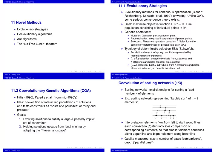
◮ E.g. sorting network representing “bubble sort” of n = 6 ◮ Idea: coevolution of interacting populations of solutions elements: and tests/constraints as “hosts and parasites” or “prey and predator” ◮ Goals: 1. Evolving solutions to satisfy a large & possibly implicit ◮ Interpretation: elements flow from left to right along lines; set of constraints each connection (“gate”) indicates comparison of 2. Helping solutions escape from local minima by corresponding elements, so that smaller element continues adapting the “fitness landscape” along upper line and bigger element along lower line ◮ Quality measures: size = number of gates (comparisons), depth (“parallel time”) I.N. & P .O. Spring 2006 I.N. & P .O. Spring 2006

  2. T–79.4201 Search Problems and Algorithms T–79.4201 Search Problems and Algorithms Coevolution of sorting networks (2/3) ◮ Quite a bit of work in the 1960’s (cf. Knuth Vol. 3); size-optimal networks known for n ≤ 8 ; for n > 8 the optimal design problem gets difficult. ◮ “Classical” challenge: n = 16 . A general construction of Batcher & Knuth (1964) yields 63 gates; this was Coevolution of sorting networks (3/3) unexpectedly beaten by Shapiro (1969) with 62 gates, and later by Green (1969) with 60 gates. (Best known network.) ◮ Result when population of test cases not evolved: 65-gate ◮ Hillis (1990): Genetic and coevolutionary genetic sorting network algorithms for the n = 16 sorting network design problem: ◮ Coevolution: ◮ Each individual represents a network with between 60 and 120 ◮ Fitness of networks = % of test cases sorted correctly gates ◮ Fitness of test cases = % of networks fooled ◮ Genetic operations defined appropriately ◮ Also population of test cases evolves using appropriate genetic ◮ Individuals not guaranteed to represent proper sorting networks; operations behaviour tested on a population of test cases ◮ Population sizes up to 65536 individuals, runs 5000 generations ◮ Result of coevolution: a novel sorting network with 61 gates: I.N. & P .O. Spring 2006 I.N. & P .O. Spring 2006 T–79.4201 Search Problems and Algorithms T–79.4201 Search Problems and Algorithms 11.3 Ant Algorithms ◮ Dorigo et al. (1991 onwards), Hoos & Stützle (1997), ... ◮ Inspired by experiment of real ants selecting the shorter of two paths (Goss et al. 1989): NEST FOOD ◮ Method: each ant leaves a pheromone trail along its path; ants make probabilistic choice of path biased by the amount of pheromone on the ground; ants travel faster along the shorter path, hence it gets a differential advantage on the amount of pheromone deposited. I.N. & P .O. Spring 2006 I.N. & P .O. Spring 2006

  3. T–79.4201 Search Problems and Algorithms T–79.4201 Search Problems and Algorithms Ant Colony Optimisation (ACO) ◮ Formulate given optimisation task as a path finding problem from source s to some set of valid destinations ◮ Have each agent distribute its pheromone reward △ τ t 1 ,..., t n (cf. the A ∗ algorithm). among edges ( i , j ) on its path π : either as τ ij ← τ ij + △ τ or ◮ Have agents (“ants”) search (in serial or parallel) for as τ ij ← τ ij + △ τ / len ( π ) . candidate paths, where local choices among edges leading ◮ Between two iterations of the algorithm, have the from node i to neighbours j ∈ N i are made probabilistically pheromone levels “evaporate” at a constant rate ( 1 − ρ ) : according to the local “pheromone distribution” τ ij : τ ij ← ( 1 − ρ ) τ ij . τ ij p ij = . ∑ j ∈ N i τ ij ◮ After an agent has found a complete path π from s to one of the t k , “reward” it by an amount of pheromone proportional to the quality of the path, △ τ ∝ q ( π ) . I.N. & P .O. Spring 2006 I.N. & P .O. Spring 2006 T–79.4201 Search Problems and Algorithms T–79.4201 Search Problems and Algorithms ◮ Several modifications proposed in the literature: (i) to exploit best solutions, allow only best agent of each iteration to distribute pheromone; (ii) to maintain diversity, set lower and upper limits on the edge pheromone levels; (iii) to speed up discovery of good paths, run some local optimisation algorithm on the paths found by the agents; ACO motivation etc. ◮ Local choices leading to several good global results get reinforced by pheromone accumulation. ◮ Evaporation of pheromone maintains diversity of search. (I.e. hopefully prevents it getting stuck at bad local minima.) ◮ Good aspects of the method: can be distributed; adapts automatically to online changes in the quality function q ( π ) . ◮ Good results claimed for Travelling Salesman Problem, Quadratic Assignment, Vehicle Routing, Adaptive Network Routing etc. I.N. & P .O. Spring 2006 I.N. & P .O. Spring 2006

  4. T–79.4201 Search Problems and Algorithms T–79.4201 Search Problems and Algorithms An ACO algorithm for the TSP (2/2) An ACO algorithm for the TSP (1/2) ◮ The local choice of moving from city i to city j is biased ◮ Dorigo et al. (1991) according to weights: ◮ At the start of each iteration, m ants are positioned at τ α ij ( 1 / d ij ) β random start cities. a ij = ∑ j ∈ N i τ α ij ( 1 / d ij ) β , ◮ Each ant constructs probabilistically a Hamiltonian tour π on the graph, biased by the existing pheromone levels. where α , β ≥ 0 are parameters controlling the balance (NB. the ants need to remember and exclude the cities between the current strength of the pheromone trail τ ij vs. they have visited during the search.) the actual intercity distance d ij . ◮ In most variations of the algorithm, the tours π are still ◮ Thus, the local choice distribution at city i is: locally optimised using e.g. the Lin-Kernighan 3-opt procedure. a ij p ij = , ◮ The pheromone award for a tour π of length d ( π ) is i a ij ∑ j ∈ N ′ △ τ = 1 / d ( π ) , and this is added to each edge of the tour: where N ′ i is the set of permissible neighbours of i after τ ij ← τ ij + 1 / d ( π ) . cities visited earlier in the tour have been excluded. I.N. & P .O. Spring 2006 I.N. & P .O. Spring 2006 T–79.4201 Search Problems and Algorithms T–79.4201 Search Problems and Algorithms 11.4 The “No Free Lunch” Theorem The NFL theorem: definitions (1/3) ◮ Wolpert & Macready 1997 ◮ Consider family F of all possible objective functions ◮ Basic content: All optimisation methods are equally good, mapping finite search space X to finite value space Y . when averaged over uniform distribution of objective ◮ A sample d from the search space is an ordered sequence functions. ◮ Alternative view: Any nontrivial optimisation method must of distinct points from X , together with some associated cost values from Y : be based on assumptions about the space of relevant objective functions. [However this is very difficult to make d = { ( d x ( 1 ) , d y ( 1 )) ,..., ( d x ( m ) , d y ( m )) } . explicit and hardly any results in this direction exist.] ◮ Corollary: one cannot say, unqualified, that ACO methods Here m is the size of the sample. A sample of size m is also are “better” than GA’s, or that Simulated Annealing is denoted by d m , and its projections to just the x - and m and d y y -values by d x “better” than simple Iterated Local Search. [Moreover as of m , respectively. now there are no results characterising some nontrivial ◮ The set of all samples of size m is thus D m = ( X × Y ) m , class of functions F on which some interesting method A and the set of all samples of arbitrary size is D = ∪ m D m . would have an advantage over, say, random sampling of the search space.] I.N. & P .O. Spring 2006 I.N. & P .O. Spring 2006

Download Presentation
Download Policy: The content available on the website is offered to you 'AS IS' for your personal information and use only. It cannot be commercialized, licensed, or distributed on other websites without prior consent from the author. To download a presentation, simply click this link. If you encounter any difficulties during the download process, it's possible that the publisher has removed the file from their server.

Recommend


More recommend