[PDF] - 1 Weights Need Not be Reals Goal: Parameterized FSMs a/ q / p b/ r PDF Document

SLIDE 1

1

Parameterized Finite-State Machines and their Training

Jason Eisner Jason Eisner

Johns Hopkins University October 16, 2002 — AT&T Speech Days

Outline – The Vision Slide!

1. Finite-state machines

as a shared modeling language.

2. The training gizmo

(an algorithm).

Should use out of-the-box finite-state gizmos to build and train most of our current models. Easier, faster, better, & enables fancier models.

Training Probabilistic FSMs

State of the world – surprising:

Training for HMMs, alignment, many variants But no basic training algorithm for all FSAs Fancy toolkits for building them, but no learning

New algorithm:

Training for FSAs, FSTs, … (collectively FSMs) Supervised, unsupervised, incompletely supervised … Train components separately or all at once Epsilon-cycles OK Complicated parameterizations OK “I f you build it, it will train” Build parts by hand For each part, get arc weights somehow Then combine parts (much more limited) Fancy regular expressions

(or sometimes TBL)

How they’re currently built Noisy channel models p(x)p(y| x)p(z| y)… (much more limited) Encode expert knowledge about Arabic morphology, etc. How they’re currently used

Prob. distributions

p(x,y) or p(y|x). Functions on strings. Or nondeterministic functions (relations). What they represent Probabilistic FSTs Vanilla FSTs

Currently Tw o Finite-State Camps

Current Limitation

Big FSM must be made of separately

trainable parts.

Knight & Graehl 1997 - transliteration p(English text) p(English text English phonemes) p(English phonemes Japanese phonemes) p(Japanese phonemes Japanese text)

Need explicit training data for this

part (smaller loanword corpus). A pity – would like to use guesses. Topology must be simple enough to train by current methods. A pity – would like to get some of that expert knowledge in here!

Topology: sensitive to syllable struct? Parameterization: /t/ and /d/ are similar phonemes … parameter tying?

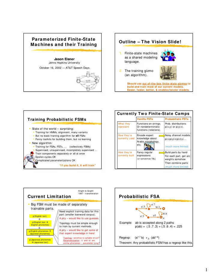
Example: ab is accepted along 2 paths p(ab) = (.5 .7 .3) + (.5 .6 .4) = .225

Probabilistic FSA

ε/.5 a/1 a/.7 b/.3 ε/.5 b/.6 .4

Regexp: (a*.7 b) +.5 (ab*.6) Theorem: Any probabilistic FSM has a regexp like this.

SLIDE 2

2

Example: ab is accepted along 2 paths weight(ab) = (p⊗ ⊗ ⊗ ⊗q⊗ ⊗ ⊗ ⊗r) ⊕ ⊕ ⊕ ⊕ (w⊗ ⊗ ⊗ ⊗x⊗ ⊗ ⊗ ⊗y⊗ ⊗ ⊗ ⊗z)

Weights Need Not be Reals

ε/p a/x a/q b/r ε/w b/y z

If If ⊗ ⊗ ⊕ ⊕ * satisfy * satisfy “ “semiring semiring” ” axioms, axioms, the finite the finite -

state constructions

state constructions continue to w ork correctly. continue to w ork correctly.

Goal: Parameterized FSMs

Parameterized FSM:

An FSM whose arc probabilities depend on

parameters: they are formulas.

ε/p a/q* exp(t+ u) a/q b/(1-q)r ε/1-p a/r 1-s a/exp(t+ v) Expert first: Construct the FSM (topology & parameterization). Automatic takes over: Given training data, find parameter values that optimize arc probs.

Goal: Parameterized FSMs

Parameterized FSM:

An FSM whose arc probabilities depend on

parameters: they are formulas.

ε/.1 a/.44 a/.2 b/.8 ε/.9 a/.3 .7 a/.56 Expert first: Construct the FSM (topology & parameterization). Automatic takes over: Given training data, find parameter values that optimize arc probs.

Goal: Parameterized FSMs

FSM whose arc probabilities are formulas.

Knight & Graehl 1997 - transliteration p(English text) p(English text English phonemes) p(English phonemes Japanese phonemes) p(Japanese phonemes Japanese text)

“Would like to get some of that

expert knowledge in here” Use probabilistic regexps like

(a*.7 b) +.5 (ab*.6) …

If the probabilities are variables

(a*x b) +y (ab*z) …

then arc weights of the compiled machine are nasty formulas. (Especially after minimization!)

Goal: Parameterized FSMs

An FSM whose arc probabilities are

formulas.

Knight & Graehl 1997 - transliteration p(English text) p(English text English phonemes) p(English phonemes Japanese phonemes) p(Japanese phonemes Japanese text)

“/t/ and /d/ are similar …”

Tied probs for doubling them:

/t/:/tt/ /d/:/dd/ p p

Goal: Parameterized FSMs

An FSM whose arc probabilities are

formulas.

Knight & Graehl 1997 - transliteration p(English text) p(English text English phonemes) p(English phonemes Japanese phonemes) p(Japanese phonemes Japanese text)

“/t/ and /d/ are similar …”

Loosely coupled probabilities:

/t/:/tt/ /d/:/dd/ exp p+ q+ r (coronal, stop, unvoiced) exp p+ q+ s (coronal, stop, voiced) (with normalization)

SLIDE 3

3

Outline of this talk

1. What can you build with

parameterized FSMs?

2. How do you train them?

p(x)

=

Finite-State Operations

Projection GIVES YOU marginal distribution

domain( p(x,y) )

p(y)

=

range(

p(x,y) )

a : b / 0.3 a : b / 0.3

0.3 p(x) + 0.7 q(x)

=

Finite-State Operations

Probabilistic union GIVES YOU mixture model

p(x)

+ 0.3

q(x) p(x) q(x)

0.3 0.7

α p(x) + (1- α)q(x)

=

Finite-State Operations

Probabilistic union GIVES YOU mixture model

p(x)

+ α

q(x) p(x) q(x)

α

1-α

Learn the mixture parameter α!

p(x| z)

=

Finite-State Operations

Composition GIVES YOU chain rule

p(x|y) o p(y|z) p(x,z)

=

z

p(x|y) o p(y|z)

The most popular statistical FSM operation Cross-product construction

Finite-State Operations

Concatenation, probabilistic closure

HANDLE unsegmented text

p(x) q(x) p(x) p(x) q(x) * 0.3

0.3 0.7

p(x)

Just glue together machines for the different

segments, and let them figure out how to align with the text

SLIDE 4

4

Finite-State Operations

Directed replacement MODELS noise or

postprocessing p(x, noisy y)

=

p(x,y)

Resulting machine compensates for noise
r postprocessing

D

noise model defined by dir. replacement

p(x)* q(x)

=

Finite-State Operations

Intersection GIVES YOU product models

e.g., exponential / maxent, perceptron, Naïve Bayes, …

p(x)

& q(x)

pNB(y | x)

∝

&

p(y) p(A(x)|y) & p(B(x)|y) &

Cross-product construction (like composition)

Need a normalization op too – computes ∑x f(x)

“pathsum” or “partition function”

Finite-State Operations

Conditionalization (new operation)

p(y | x)

=

condit( p(x,y) ) p(x,y)

Construction:

reciprocal(determinize(domain( ))) o p(x,y)

not possible for all weighted FSAs

Resulting machine can be composed with

ther distributions: p(y | x) * q(x)

Other Useful Finite-State Constructions

Complete graphs YIELD n-gram models Other graphs YIELD fancy language models (skips, caching, etc.) Compilation from other formalism FSM: Wordlist (cf. trie), pronunciation dictionary ... Speech hypothesis lattice Decision tree (Sproat & Riley) Weighted rewrite rules (Mohri & Sproat) TBL or probabilistic TBL (Roche & Schabes) PCFG (approximation!) (e.g., Mohri & Nederhof) Optimality theory grammars (e.g., Eisner) Logical description of set (Vaillette; Klarlund)

Regular Expression Calculus as a Modelling Language

Function Function on strings,

r probability distrib.

Source code Regular expression (can be probabilistic) Object code Finite state machine Compiler Regexp compiler Optimization of

bject code

Determinization, minimization, pruning

Programming Languages The Finite-State Case

Regular Expression Calculus as a Modelling Language

Function composition Machine composition Nondeterminism Nondeterminism Parallelism Compose FSA with FST Function inversion (cf. Prolog) Function inversion Higher-order functions Transform object code (apply operators to it) Many features you wish other languages had!

Programming Languages The Finite-State Case

SLIDE 5

5

Regular Expression Calculus as a Modelling Language

Statistical FSMs still done in assembly language

Build machines by manipulating arcs and states For training,

get the weights by some exogenous procedure and patch them onto arcs you may need extra training data for this you may need to devise and implement a new variant of EM

Would rather build models declaratively ((a*.7 b) +.5 (ab*.6)) ° repl.9((a:(b +.3 ε))*,L,R)

Outline

1. What can you build with

parameterized FSMs?

2. How do you train them?

Hint: Make the finite-state machinery do the work.

How Many Parameters?

Final machine p(x,z) But really I built it as p(x,y) o p(z|y) 17 weights – 4 sum-to-one constraints = 13 apparently free parameters 5 free parameters 1 free parameter

How Many Parameters?

But really I built it as p(x,y) o p(z|y) 5 free parameters 1 free parameter Even these 6 numbers could be tied ...

r derived by formula from

a smaller parameter set.

How Many Parameters?

But really I built it as p(x,y) o p(z|y) 5 free parameters 1 free parameter Really I built this as

(a:p)*.7 (b: (p +.2 q))*.5

3 free parameters

Training a Parameterized FST

Given: an expression (or code) to build the FST from a parameter vector θ 1. Pick an initial value of θ 2. Build the FST – implements fast prob. model 3. Run FST on some training examples to compute an objective function F(θ) 4. Collect E-counts or gradient ∇F(θ) 5. Update θ to increase F(θ) 6. Unless we converged, return to step 2

SLIDE 6

6

x1 y1 y2 y1 x2 x1 x3 x2 x1 y3 y2 y1

Training a Parameterized FST

(our current FST, reflecting our current guess of the parameter vector)

… …

At each training pair (xi, yi), collect E counts or gradients that indicate how to increase p(xi, yi). T =

What are x i and yi?

xi yi

T = (our current FST, reflecting our current guess of the parameter vector)

What are x i and yi?

xi = banana yi = bandaid

T = (our current FST, reflecting our current guess of the parameter vector)

What are x i and yi?

xi = yi = b a n a n a b a n d a i d

T = (our current FST, reflecting our current guess of the parameter vector) fully supervised

What are x i and yi?

xi = yi = b a n a b a n d a i d

ε ε ε ε

loosely supervised T = (our current FST, reflecting our current guess of the parameter vector)

What are x i and yi?

yi = b a n d a i

unsupervised, e.g., Baum-Welch. Transition seq xi is hidden Emission seq yi is observed

d xi = Σ

Σ Σ Σ* = Σ Σ Σ Σ

T = (our current FST, reflecting our current guess of the parameter vector)

SLIDE 7

7

Building the Trellis

xi = yi =

T = Extracts paths from T that are compatible with (xi, yi). Tends to unroll loops of T, as in HMMs, but not always.

xi o T o yi =

COMPOSE to get trellis:

Summing the Trellis

Extracts paths from T that are compatible with (xi, yi). Tends to unroll loops of T, as in HMMs, but not always.

xi o T o yi =

Let ti = total probability of all paths in trellis = p(xi, yi) This is what we want to increase! How to compute ti? If acyclic (exponentially many paths): dynamic programming. If cyclic (infinitely many paths): solve sparse linear system.

xi, yi are regexps (denoting strings or sets of strings)

epsilonify ( xi o T o yi )

Remark: In principle, FSM minimization algorithm already knows how to compute ti, although not the best method.

Summing the Trellis

xi o T o yi =

Let ti = total probability of all paths in trellis = p(xi, yi). This is what we want to increase!

minimize ( ) =

ti replace all arc labels with ε

Mama/.05 Mama/.005 Mama Iwant/.0005 Mama Iwant Iwant/.00005

Example: Baby Think & Baby Talk

ε:m/.05 Mama:m IWant:ε /.1 IWant:u/.8 .1 .1 IWant:ε /.1 m m

bserve
bserve

talk talk recover recover think, by think, by composition composition

ε:m/.05 Mama:m X:m/.4 X:m/.4 .2 XX/.032 Total = .0375555555 X:b/.2 X:m/.4 .2

Joint Prob. by Double Composition

ε:m/.05 Mama:m X:b/.2 X:m/.4 .2 IWant:ε /.1 IWant:u/.8 .1 m m

talk talk compose compose

.1 IWant:ε /.1 ε:m/.05 Mama:m X:m/.4 X:m/.4 .2

think think

Σ Σ Σ Σ

p(Σ Σ Σ Σ* : mm) = .0375555 = sum of paths

Joint Prob. by Double Composition

ε:m/.05 Mama:m X:b/.2 X:m/.4 .2 IWant:ε /.1 IWant:u/.8 .1 m m

talk talk compose compose

.1 ε:m/.05 Mama:m

think think

p(Σ Σ Σ Σ* : mm) = .0005 = sum of paths

Mama IWant IWant:ε /.1

SLIDE 8

8

Joint Prob. by Double Composition

ε:m/.05 Mama:m X:b/.2 X:m/.4 .2 IWant:ε /.1 IWant:u/.8 .1 m m

talk talk compose compose

.1 IWant:ε /.1 ε:m/.05 Mama:m X:m/.4 X:m/.4 .2

think think

Σ Σ Σ Σ

p(Σ Σ Σ Σ* : mm) = .0375555 = sum of paths

Summing Over All Paths

ε:m/.05 Mama:m X:b/.2 X:m/.4 .2 IWant:ε /.1 IWant:u/.8 .1 m:ε m:ε

talk talk compose compose

.1 ε:ε/.1 ε:ε/.05 ε:ε ε:ε/.4 ε:ε/.4 .2

think think

ε:Σ Σ Σ Σ

p(Σ Σ Σ Σ* : mm) = .0375555 = sum of paths

Summing Over All Paths

ε:m/.05 Mama:m X:b/.2 X:m/.4 .2 IWant:ε /.1 IWant:u/.8 .1 m:ε m:ε

talk talk compose compose + minimize + minimize think think

ε:Σ Σ Σ Σ

p(Σ Σ Σ Σ* : mm) = .0375555 = sum of paths

0.0375555

Where We Are Now

“minimize (epsilonify ( xi o T o yi ) )” =

ti

ε ε ε ε/

btains ti = sum of trellis paths = p(xi, yi).

Want to change parameters to make ti increase.

Solution: Annotate every probability with bookkeeping info. So probabilities know how they depend on parameters. Then the probability ti will know, too! It will emerge annotated with info about how to increase it. The machine T is built with annotations from the ground up. a vector

Example: ab is accepted along 2 paths p(ab) = (.5 .7 .3) + (.5 .6 .4) = .225

Probabilistic FSA

ε/.5 a/1 a/.7 b/.3 ε/.5 b/.6 .4

Regexp: (a*.7 b) +.5 (ab*.6) Theorem: Any probabilistic FSM has a regexp like this. Example: ab is accepted along 2 paths weight(ab) = (p⊗ ⊗ ⊗ ⊗q⊗ ⊗ ⊗ ⊗r) ⊕ ⊕ ⊕ ⊕ (w⊗ ⊗ ⊗ ⊗x⊗ ⊗ ⊗ ⊗y⊗ ⊗ ⊗ ⊗z)

Weights Need Not be Reals

ε/p a/x a/q b/r ε/w b/y z

If If ⊗ ⊗ ⊕ ⊕ * satisfy * satisfy “ “semiring semiring” ” axioms, axioms, the finite the finite -

state constructions

state constructions continue to w ork correctly. continue to w ork correctly.

SLIDE 9

9

p ⊗ ⊗ ⊗ ⊗ q

Intersect, Compose: ⊗

p*

Closure: *

p ⊗ ⊗ ⊗ ⊗ q

Concat: ⊗

p ⊕ ⊕ ⊕ ⊕ q

Union: ⊕

Weight of a string is total weight of its accepting paths.

Semiring Definitions

p q p q p p q

p ⊗ ⊗ ⊗ ⊗ q = pq

Intersect, Compose: ⊗

p* = 1+p+p2 + … = (1-p)-1

Closure: *

p ⊗ ⊗ ⊗ ⊗ q = pq

Concat: ⊗

p ⊕ ⊕ ⊕ ⊕ q = p+q

Union: ⊕

Weight of a string is total weight of its accepting paths.

The Probability Semiring

p q p q p p q

(p,x) ⊗ ⊗ ⊗ ⊗ (q,y) = (pq, py + qx)

Intersect, Compose: ⊗

(p,x)* = ((1-p)-1, (1-p)-2x)

Closure: *

(p,x) ⊗ ⊗ ⊗ ⊗ (q,y) = (pq, py + qx)

Concat: ⊗

(p,x) ⊕ ⊕ ⊕ ⊕ (q,y) = (p+q, x+y)

Union: ⊕

The (Probability, Gradient) Semiring

p,x q,y p,x q,y p,x p,x q,y

where p is gradient

Base case

p, p

We Did It!

We now have a clean algorithm for

computing the gradient.

xi o T o yi =

How to compute ti? Just like before, when ti = p(xi, yi). But in new semiring. If acyclic (exponentially many paths): dynamic programming. If cyclic (infinitely many paths): solve sparse linear system. Or can always just use minimize ( epsilonify (xi o T o yi ) ). Let ti = total annotated probability of all paths in trellis = (p(xi, yi), p(xi, yi)). Aggregate over i (training examples).

An Alternative: EM

Would be easy to train probabilities if we’d seen the paths the machine followed

1. E-step: Which paths probably generated the
bserved data? (according to current probabilities)
2. M-step: Reestimate probabilities (or θ) as if those

guesses were right

3. Repeat

Guaranteed to converge to local optimum.

Mama/.005 Mama Iwant/.0005 Mama Iwant Iwant/.00005 .1 IWant:ε /.1

paths consistent with (xi,yi)

ε:m/.05 Mama:m X:m/.4 X:m/.4 .2 XX/.032 Total = .0375555555 ε:m/.05 Mama:m X:b/.2 X:m/.4 .2 IWant:ε /.1 IWant:u/.8 .1 m m

talk think

Σ Σ Σ Σ

x x i

i

T T y yi

i

Baby Says mm

SLIDE 10

10

Which Arcs Did We Follow ?

p(mm) = p(Σ Σ Σ Σ* : mm) = .0375555 = sum of all paths p(Mama : mm) = .005 p(Mama Iwant : mm) = .0005 p(Mama Iwant Iwant : mm) = .00005 etc. p(XX : mm) = .032 p(Mama | mm) = .005/.037555 = 0.13314 p(Mama Iwant | mm) = .0005/.037555 = 0.01331 p(Mama Iwant Iwant | mm) = .00005/.037555 = 0.00133 p(XX | mm) = .032/.037555 = 0.85207 relative probs. .1 IWant:ε /.1 ε:m/.05 Mama:m X:m/.4 X:m/.4 .2

paths consistent with (Σ

Σ Σ Σ*, mm)

Count Uses of Original Arcs

p(Mama | mm) = .005/.037555 = 0.13314 p(Mama Iwant | mm) = .0005/.037555 = 0.01331 p(Mama Iwant Iwant | mm) = .00005/.037555 = 0.00133 p(XX | mm) = .032/.037555 = 0.85207 relative probs. .1 IWant:ε /.1 ε:m/.05 Mama:m X:m/.4 X:m/.4 .2

paths consistent with (Σ

Σ Σ Σ*, mm)

ε:m/.05 Mama:m X:b/.2 X:m/.4 .2 IWant:ε /.1 IWant:u/.8 .1

paths consistent with (Σ

Σ Σ Σ*, mm)

ε:m/.05 Mama:m X:b/.2 X:m/.4 .2 IWant:ε /.1 IWant:u/.8 .1

Count Uses of Original Arcs

p(Mama | mm) = .005/.037555 = 0.13314 p(Mama Iwant | mm) = .0005/.037555 = 0.01331 p(Mama Iwant Iwant | mm) = .00005/.037555 = 0.00133 p(XX | mm) = .032/.037555 = 0.85207 relative probs. ε:m/.05 Mama:m X:b/.2 X:m/.4 .2 IWant:ε /.1 IWant:u/.8 .1

Expect 0.85207 × 2 traversals of

riginal arc

(on example Σ

Σ Σ Σ*, mm)

.1 IWant:ε /.1 ε:m/.05 Mama:m X:m/.4 X:m/.4 .2

.1/b3 .8/b5

b1 = (1,0,0,0,0,0,0) b4 = (0,0,0,1,0,0,0) b7 = (0,0,0,0,0,0,1) b2 = (0,1,0,0,0,0,0) b5 = (0,0,0,0,1,0,0) b3 = (0,0,1,0,0,0,0) b6 = (0,0,0,0,0,1,0)

Expected-Value Formulation

.05/b4 1/0 .3/b1 .4/b2 .1/b6 .1/b7

T =

Associate a value with each arc we wish to track

.1/b3 .8/b5

b1 = (1,0,0,0,0,0,0) b4 = (0,0,0,1,0,0,0) b7 = (0,0,0,0,0,0,1) b2 = (0,1,0,0,0,0,0) b5 = (0,0,0,0,1,0,0) b3 = (0,0,1,0,0,0,0) b6 = (0,0,0,0,0,1,0)

Expected-Value Formulation

.05/b4 1/0 .3/b1 .4/b2 .1/b6 .1/b7

T =

Associate a value with each arc we wish to track

xi o T o yi =

.4/b2 .4/b2 .1/b3

has total value b2 + b2 + b3 = (0,2,1,0,0,0,0) Tells us the observed counts of arcs in T.

Expected-Value Formulation

Associate a value with each arc we wish to track

xi o T o yi =

.4/b2 .4/b2 .2/b3

has total value b2 + b2 + b3 = (0,2,1,0,0,0,0) Tells us the observed counts of arcs in T.

But what if xi o T o yi had multiple paths? We want the expected path value for the E step of EM. Some paths more likely than others.

expected value = Σ value(path) p(path | xi, yi) = Σ value(path) p(path) / Σ p(path)

We’ll arrange for ti = (Σ p(path), Σ value(path) p(path))

SLIDE 11

11

where v is arc value

Base case

(p,x) ⊗ ⊗ ⊗ ⊗ (q,y) = (pq, py + qx)

Intersect, Compose: ⊗

(p,x)* = ((1-p)-1, (1-p)-2x)

Closure: *

(p,x) ⊗ ⊗ ⊗ ⊗ (q,y) = (pq, py + qx)

Concat: ⊗

(p,x) ⊕ ⊕ ⊕ ⊕ (q,y) = (p+q, x+y)

Union: ⊕

The Expectation Semiring

p,x q,y p,x q,y p,x p,x q,y p, pv

ti = (Σ p(path), Σ value(path) p(path))

same as before!

That’s the algorithm!

Existing mechanisms do all the work Keeps count of original arcs despite composition, loop unrolling, etc. Cyclic sums handled internally by the minimization step, which heavily uses semiring closure operation Flexible: can define arc values as we like

Example: Log-linear (maxent) parameterization
M-step: Must reestimate θ from feature counts (e.g., Iterative Scaling)
If arc’s weight is exp(θ2+θ5), let its value be (0,1,0,0,1, ...)
Then total value of correct path for (xi,yi) – counts observed features
E-step: Needs to find expected value of path for (xi,yi)

Log-Linear Parameterization

Some Optimizations

Exploit (partial) acyclicity Avoid expensive vector operations Exploit sparsity Rebuild quickly after parameter update

xi o T o yi =

Let ti = total annotated probability of all paths in trellis = (p(xi, yi), bookkeeping information).

Need Faster Minimization

Hard step is the minimization:

Want total semiring weight of all paths Weighted ε-closure must invert a semiring matrix

Want to beat this! (takes O(n3) time) Optimizations exploit features of problem

.1 ε:ε/.1 ε:ε/.05 ε:ε ε:ε/.4 ε:ε/.4 .2

All-Pairs vs. Single-Source

For each q, r, ε-closure finds total weight of all q r paths But we only need total weight of init final paths Solve linear system instead of inverting matrix: Let α(r) = total weight of init r paths α(r) = ∑q α(q) * weight(q → r) α(init) = 1 + ∑q α(q) * weight(q → init) But still O(n3) in worst case

SLIDE 12

12

Cycles Are Usually Local

In HMM case, Ti = (ε × xi) o T o (yi × ε) is an acyclic lattice: Acyclicity allows linear-time dynamic

programming to find our sum over paths

If not acyclic, first decompose into minimal

cyclic components (Tarjan 1972, 1981; Mohri 1998)

Now full O(n3) algorithm must be run for several small n instead of one big n – and reassemble results More powerful decompositions available (Tarjan 1981);

block-structured matrices

Avoid Semiring Operations

Our semiring operations aren’t O(1)

They manipulate vector values

To see how this slows us down, consider HMMs: Our algorithm computes sum over paths in lattice.

If acyclic, requires a forward pass only.

Where’s backward pass? What we’re pushing forward is (p,v)

Arcs v go forward to be downweighted by later probs, instead of probs going backward to downweight arcs. The vector v rapidly loses sparsity, so this is slow!

We’re already computing forward probabilities α(q) Also compute backward probabilities β(r)

Avoid Semiring Operations

p Total probability of paths through this arc = α(q) * p * β(r) E[path value] = ∑q,r (α(q) * p(q → r) * β(r)) * value(q → r) Exploits structure of semiring Now α, β are probabilities, not vector values q

α(q)

r β(r)

Avoid Semiring Operations

Now our linear systems are over the reals: Let α(r) = total weight of init r paths α(r) = ∑q α(q) * weight(q → r) α(init) = 1 + ∑q α(q) * weight(q → init) Well studied! Still O(n3) in worst case, but:

Proportionately faster for sparser graph

Approximate solutions possible

Relaxation (Mohri 1998) and back-relaxation (Eisner 2001); or stop iterative method earlier

Lower space requirement: O(|states|) vs. O(|states|2)

Fast Updating

1. Pick an initial value of θ 2. Build the FST – implements fast prob. model ... 6. Unless we converged, return to step 2

But step 2 might be slow! Recompiles the FST from its parameterized regexp, using the new parameters θ. This involves a lot of structure-building, not just arithmetic

Matching arc labels in intersection and composition Memory allocation/deallocation Heuristic decisions about time-space tradeoffs

Fast Updating

Solution: Weights remember underlying formulas A weight is a pointer into a formula DAG

exp +

θ5

0.3 1

2

*

θ2 θ1

0.135 0.04

3

+

*

0.7 θ8 0.21 0.345

may or may not be used in obj. function; update on demand

Each node caches its current value When (some) parameters are updated, invalidate (some) caches Similar to a heap Allows approximate updates

SLIDE 13

13

Easy to experiment with interesting models. Change a model = edit declarative specification Combine models = give a simple regexp Train the model = push a button Share your model = upload to archive Speed up training = download latest version

(conj gradient, pruning …)

Avoid local maxima = download latest version

(deterministic annealing …) p.s. Expectation semirings extend naturally to context-free case, e.g., Inside-Outside algorithm.

The Sunny Future

Marrying Tw o Finite-State Traditions

Classic stat models & Classic stat models & variants variants ⇒ ⇒ simple simple FSMs FSMs

HMMs, edit distance, sequence alignment, n-grams, segmentation

Expert know ledge Expert know ledge ⇒ ⇒ hand hand-

crafted

crafted FSMs FSMs

Extended regexps, phonology/morphology, info extraction, syntax … Design Design complex finite complex finite -

state model for task

state model for task Any extended regexp Any machine topology; epsilon-cycles ok Parameterize Parameterize as desired to make it probabilistic as desired to make it probabilistic Combine models freely, tying parameters at will Then find best Then find best param param values from data (by EM or CG) values from data (by EM or CG)

Trainable from data Tailored to task Tailor model, then train end-to-end

Ways to Improve Toolkit

Experiment with other learning algs …

Conjugate gradient is a trivial variation; should be faster Annealing etc. to avoid local optima

Experiment with other objective functions …

Trivial to incorporate a Bayesian prior Discriminative training: maximize p(y | x), not p(x,y)

Experiment with other parameterizations …

Mixture models Maximum entropy (log-linear): track expected feature counts, not arc counts

Generalize more: Incorporate graphical modelling

Some Applications

Prediction, classification, generation; more generally, “filling in of blanks”

Speech recognition Machine translation, OCR, other noisy-channel models Sequence alignment / Edit distance / Computational biology Text normalization, segmentation, categorization Information extraction Stochastic phonology/morphology, including lexicon Tagging, chunking, finite-state parsing Syntactic transformations (smoothing PCFG rulesets)

Quickly specify & combine models Tie parameters & train end-to-end Unsupervised, partly supervised, erroneously supervised

FIN

that’s all folks (for now)

wish lists to eisner@cs.jhu.edu