1 Simple example of simulation Slide 4 Evaluation of expected - PDF document

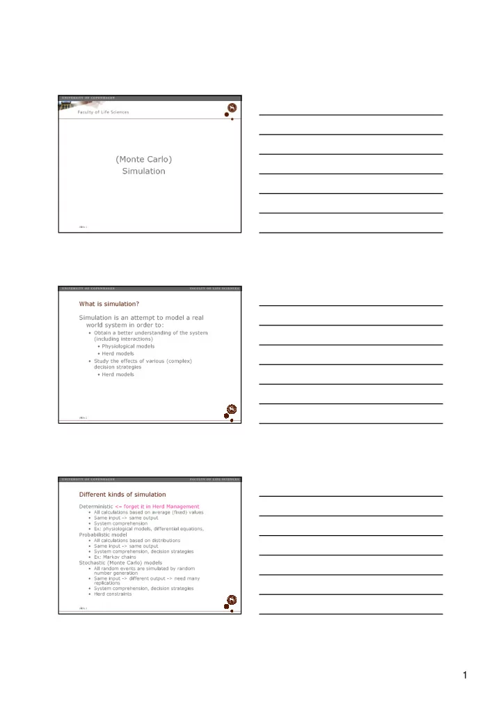
(Monte Carlo) Simulation (Monte Carlo) Simulation Slide 1 What is simulation? Simulation is an attempt to model a real world system in order to: • Obtain a better understanding of the system (including interactions) • Physiological models • Herd models • Study the effects of various (complex) decision strategies • Herd models Slide 2 Different kinds of simulation Deterministic <– forget it in Herd Management • All calculations based on average (fixed) values • Same input -> same output • System comprehension • Ex: physiological models, differential equations, Probabilistic model • All calculations based on distributions • Same input -> same output • System comprehension, decision strategies • Ex: Markov chains Stochastic (Monte Carlo) models • All random events are simulated by random number generation • Same input -> different output -> need many replications • System comprehension, decision strategies • Herd constraints Slide 3 1

Simple example of simulation Slide 4 Evaluation of expected value of production E(V) Deterministic: Simple stochastic: • Simulate 100 items with µ = 10, repeat 1000 times • E(V) = 435.60 SD = 18.73 Stochastic • Draw µ from N(10,1), simulate 100 items • Repeat the above 10.000 times • E(V) = 426.89 SD = 73.86 Slide 5 Consequence of uncertainty 0.020 Remember: magenta line 0.015 illustrates what we know! Fixed mean Stochastic mean Density 0.010 0.005 0.000 0 100 200 300 400 500 600 Value of production Slide 6 2

Different kinds of simulation (cont’d) Hierarchy • Mechanistic • A system is modeled by its elements (sub-systems) • Ex: A farm consists of buildings and a herd, the herd consists of individual cows, etc. • Empirical • Output directly modeled from the input Time • Dynamic • Ex: A herd is followed over years to evaluate the effect of a change in replacement policy, time is modeled as a variable • Static • Ex: Simulating a milking parlor with respect to capacity for a single milking Slide 7 When to use simulation? When other methods fail • Because of complexity Slide 8 The TV-show Quiz example To help formalize the concepts, we will reintroduce the old example of the TV-show Quiz with the three doors: • The host will show you 3 doors. Behind one of the doors a prize is hidden. You just have to choose the correct door to claim the prize. However, after use you choose a door, the host will open one of the other doors, always one where the treasure is not hidden. You now have the choice between : 1) keeping your initial selection; 2) changing your selection to the other unopened door. • What is the optimal strategy? You have solved this a couple of times already, but here we try with simulation. Slide 9 3

Model the quiz Choice 1 Assume: equal probability for each Opened Choice 2 door hiding the prize Gain True Slide 10 Model the quiz – identifying components Variables: • True place: ‘True’ = {1,2,3} • First choice: ‘Choice 1’ = {1,2,3} • Door opened: ‘Open’ = {1,2,3} <- Do we need that? • Second choice: ‘Choice 2’ = {‘keep’;’change’} • Reward: ‘Reward’ = {0,1000} Decision strategies: • ‘Choice 1’: Random; ‘Choice 2’=‘keep’ • ‘Choice 1’: Random; ‘Choice 2’=‘change’ • (‘Choice 1’ = 1; ‘Choice 2’ = ‘keep’ if ‘Open’ = 3 else ‘Choice 2’ = ‘change’) • (And the list goes on and on and on) Slide 11 Simulating the quiz – What do we need? We need a method for random sampling from the set {1,2,3}. A method: place the same number of green, yellow and magenta marbles in a brown paperback. Assign a number to each color and start drawing with replacement. Other methods: use a fair dice, flip a coin or … But: • “The generation of random numbers is too important to be left to chance” Use pseudo-random numbers generated by computers, so that we can reproduce the results. Motivation for that: to ensure that changes in output are truly due to changes in the model and not random variation Slide 12 4

Simulate the quiz – step-by-step • First randomly draw a door for ‘True’ e.g. 2 • Then randomly select ‘Choice 1’ e.g. 1 • Evaluate decision strategy: • ‘Choice 2’ = ‘keep’ then ‘Reward’ = 0 • ‘Choice 2’ = ‘Change’ then ‘Reward’ = 1000 • Repeat this 1000 times for each decision strategy • Calculate the average gain of each • Select the best! • And we are done… (Show Demo + R) Slide 13 Formal concepts The system consists of three parts: • Model input: • A set of decision rules Θ • A set of parameters Φ • A set of output variables Ω The parameter set can be further divided into Φ = { Φ 0 ; Φ S } Φ 0 : ‘state-of-nature’ – initial settings • Φ S : parameters that change during simulation • Φ S = [ Φ s1 , Φ s2 ,…, Φ sT ] where T is the number of • stages in the planning horizon Ω is often a subset of Φ Slide 14 Formal concepts – The TV show Quiz Model input: • A set of decision rules Θ • {‘choice 2’ = ‘keep’; ‘choice 2’ = ’change’} • A set of parameters Φ = { Φ 0 ; Φ S } Φ 0 : ‘state-of-nature’ – initial settings • • p ’true’ = (1/3;1/3;1/3) • p ’choice 1’ = (1/3;1/3;1/3) Φ S : parameters that change during simulation • • ‘true’, ‘choice 1’, ‘opened’, ’gain’ • A set of output variables Ω • ‘gain’ So, here Ω is a subset of Φ Slide 15 5

Purpose of the simulation Calculate the expected utility E(U( θ , Φ )) for each decision rule θ �\ Θ , select the one that maximizes the expected utility. • TV-Show: Expected utility ( or reward) for each of the two decision rules Expected utility: U is the utility function, but it can in general be any function of the output variables. The f-functions are density functions Slide 16 TV-show again – Integral expression The components: Φ = { p ’true’ ; p ’choice 1’ ; ‘true’, ‘choice 1’, • ‘opened’, ’gain’) • So one sample for θ 1 = ‘change’ could be: • φ i = ( p ’true’ ; p ’choice 1’ ;1,1,2,0) • U( θ 1 , φ i ) = 0 The integral is horrible, but we can easily sample from the joint distribution and evaluate the utility function Slide 17 Finally – we introduce the Monte Carlo part • Even for TV show problem the integral is more hassle to solve than it is worth. • However, sampling from the distribution followed by evaluation of the utility function is not that hard • joint distribution for ( θ , Φ ) calculate the expected So the trick: Sample a lot (e.g K ) samples from the utility as: This is the Monte Carlo part – a method for numerical integration Slide 18 6

State of nature: Favorite doors So far we assumed all doors were equal • Now, assume that host places reward behind door 1 with 80% and 10% behind each of the others • Why does it not matter? • P(succes) = P(true=1)P(choice=1) + P(true=2)P(choice=2) + P(true=3)P(choice=3) = 0.8*1/3+0.1*1/3+0.1*1/3 = 1/3 • What if you also have door 1 as favorite, 50% vs. 25% for each of the others • P(succes) = P(true=1)P(choice=1) + P(true=2)P(choice=2) + P(true=3)P(choice=3) = 0.8*0.5+0.1*0.25+0.1*0.25 Slide 19 State of nature in general State of nature will influence the optimal decision rule as well as the expected result What is the state of nature in a livestock simulation model: • Average growth rate • Herd mortality rate • Average milk yield Is the true state of nature known (with certainty) • Does it matter? • Yes, remember the simple example Slide 20 Consequence of uncertainty 0.020 Remember: magenta line 0.015 illustrates what we know! Fixed mean Stochastic mean Density 0.010 0.005 0.000 0 100 200 300 400 500 600 Value of production Slide 21 7

State of nature, livestock models • In livestock models we never know the true state of nature • We need to represent the uncertainty of the state of nature of our herd • We have some ideas: belief in the true value • The belief may be represented as a (hyper) distribution i.e. w i ~ N( µ ,2 2 ) with µ ~ N(10,1 2 ) • Representing the uncertainty of the state of nature is essential, but often ignored the consequence is that models should be seen more as research tools than means of optimizing decision rules at a specific farm Slide 22 A fresh look at the integral Slide 23 Simulation procedure Select a set of decision rules Θ to be tested For each decision rule θ �\ Θ • Draw n states of nature Φ 0 1 , .. Φ 0 n from the underlying distribution of state of nature p Φ 0 • For each state of nature Φ 0 i : • Run the simulation m times • Calculate the average result U i over the m simulations (Monte Carlo integration of the inner integral) • Calculate the average value of U 1 , U 2 , U n (Monte Carlo integration of the outer integral) Select the best performing decision rule Slide 24 8