1 Problem Statement Problem Statement Muybridge Muybridge start - - PDF document

SLIDE 1

1

Massachusetts Institute of Technology

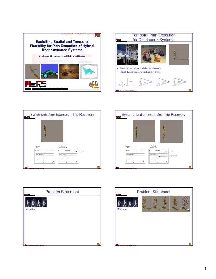
Exploiting Spatial and Temporal Flexibility for Plan Execution of Hybrid, Under-actuated Systems

Andreas Hofmann and Brian Williams

t y & y

Temporal Plan Execution for Continuous Systems

• Plan temporal and state constraints
• Plant dynamics and actuation limits

Disturbance displaces trajectory Disturbance displaces trajectory

Goal

u t l

g ≤

≤

Synchronization Example: Trip Recovery

Forward CM t goal region nominal delayed t1 t nominal t1 goal region pos. Forward stepping foot

Synchronization Example: Trip Recovery

Forward CM t goal region nominal delayed t1 t nominal t1 goal region compensated pos. Forward stepping foot

Problem Statement

Muybridge

Problem Statement

Left Foot [t_lb, t_ub] CM Right Foot start finish right toe-off right heel-strike left toe-off left heel-strike

1 l lf ∈ 1 r rf ∈

2 r rf ∈ 2 r rf ∈ 2 l lf ∈ 1 cm cm∈

Muybridge

SLIDE 2

2

Problem Statement

Left Foot [t_lb, t_ub] CM Right Foot start finish right toe-off right heel-strike left toe-off left heel-strike

1 l lf ∈ 1 r rf ∈

2 r rf ∈ 2 r rf ∈ 2 l lf ∈ 1 cm cm∈

Muybridge Qualitative State Plan

Problem Statement

Muybridge Qualitative State Plan

Left Foot [t_lb, t_ub] CM Right Foot start finish right toe-off right heel-strike left toe-off left heel-strike

1 l lf ∈ 1 r rf ∈

2 r rf ∈ 2 r rf ∈ 2 l lf ∈ 1 cm cm∈

Problem Statement

Muybridge Qualitative State Plan

Left Foot [t_lb, t_ub] CM Right Foot start finish right toe-off right heel-strike left toe-off left heel-strike

1 l lf ∈ 1 r rf ∈

2 r rf ∈ 2 r rf ∈ 2 l lf ∈ 1 cm cm∈

Problem Statement

Muybridge Qualitative State Plan

Left Foot [t_lb, t_ub] CM Right Foot start finish right toe-off right heel-strike left toe-off left heel-strike

1 l lf ∈ 1 r rf ∈

2 r rf ∈ 2 r rf ∈ 2 l lf ∈ 1 cm cm∈

Problem Statement

Muybridge Qualitative State Plan

Left Foot [t_lb, t_ub] CM Right Foot start finish right toe-off right heel-strike left toe-off left heel-strike

1 l lf ∈ 1 r rf ∈

2 r rf ∈ 2 r rf ∈ 2 l lf ∈ 1 cm cm∈

Problem Statement

Muybridge Qualitative State Plan

Left Foot [t_lb, t_ub] CM Right Foot start finish right toe-off right heel-strike left toe-off left heel-strike

1 l lf ∈ 1 r rf ∈

2 r rf ∈ 2 r rf ∈ 2 l lf ∈ 1 cm cm∈

SLIDE 3

3

Problem Statement

? u

des

CM

( ) ( )

u x, h u x, f x ≤ = &

Plant

Left Foot [t_lb, t_ub] CM Right Foot start finish right toe-off right heel-strike left toe-off left heel-strike

1 l lf ∈ 1 r rf ∈

2 r rf ∈ 2 r rf ∈ 2 l lf ∈ 1 cm cm∈

Muybridge Qualitative State Plan

Problem Statement

? u

des

CM

( ) ( )

u x, h u x, f x ≤ = &

Plant

Left Foot [t_lb, t_ub] CM Right Foot start finish right toe-off right heel-strike left toe-off left heel-strike

1 l lf ∈ 1 r rf ∈

2 r rf ∈ 2 r rf ∈ 2 l lf ∈ 1 cm cm∈

Muybridge Qualitative State Plan

Compute u such that resulting state trajectory satisfies plan

• state constraints
• temporal constraints

Problem Statement

– Achieve state-space and temporal goals specified in plan – Achieve robustness by exploiting plan flexibility – Detect plan failure as early as possible

• Challenges

– High dimensionality – Actuation limits – Interaction of limits from plan with limits of plant

CM

ZMP

horz

f

vert

f gr

f

Base of support Planner Dispatcher Skills Library A B C D [20, 30] Turn right, go forward Go forward at 1 m/s

Key Innovations

Temporal plan executive

Planner Dispatcher Skills Library A B C D [20, 30] Turn right, go forward Go forward at 1 m/s

Key Innovations

Robust to temporal disturbances Ignores continuous dynamics

Temporal plan executive

Planner Dispatcher Skills Library A B C D [20, 30] Turn right, go forward Go forward at 1 m/s

Key Innovations

t Left knee t Left hip pitch

High impedance tracking

Takes continuous dynamics into account Not flexible to disturbances

Temporal plan executive

Robust to temporal disturbances Ignores continuous dynamics

SLIDE 4

4

Key Innovations

t Left knee t Left hip pitch

High impedance tracking Model-based executive Takes continuous dynamics into account Uses plan flexibility to handle state and temporal disturbances

Planner Dispatcher Skills Library A B C D [20, 30] Turn right, go forward Go forward at 1 m/s

Temporal plan executive

Robust to temporal disturbances Ignores continuous dynamics Takes continuous dynamics into account Not flexible to disturbances

Roadmap

• Introduction

– Problem statement, innovations

• Background and approach

– Temporal plan execution systems – Robot trajectory tracking systems – Flow tubes

• Architecture and implementation
• Results
• Summary

Temporal Plan Execution Systems

• Activity plan consists of events and activities.
• Activities have temporal constraints.

A B C A B C

8 1

• 1

[0,8] [1,1] a. b.

A B C

8 1

• 1

c. 9

• 1
• Activity plan consists of events and activities.
• Activities have temporal constraints.
• Activity plan compiled into distance, dispatchable graph

[Muscettola, 1998].

A B C A B C

8 1

• 1

[0,8] [1,1] a. b.

A B C

8 1

• 1

c. 9

• 1

Temporal plan execution systems

1. Initialize execution windows.

A B C

[0,0]

a. T=0

10 10

• 5
• 1

[1,10] [6,20]

A B C

[0,0]

b. T=7

10 10

• 5
• 1

[7,7] [12,17]

A B C

[0,0]

c. T=15

10 10

• 5
• 1

[7,7] [15,15]

Temporal plan dispatcher

1. Initialize execution windows. 2. Schedule next event.

• Set event execution time to valid time

in window

3. Wait until event time.

A B C

[0,0]

a. T=0

10 10

• 5
• 1

[1,10] [6,20]

A B C

[0,0]

b. T=7

10 10

• 5
• 1

[7,7] [12,17]

A B C

[0,0]

c. T=15

10 10

• 5
• 1

[7,7] [15,15]

• Ex. Event time for B = 7

Temporal plan dispatcher

SLIDE 5

5

1. Initialize execution windows. 2. Schedule next event.

• Set event execution time to valid time

in window

3. Wait until event time. 4. Update execution windows.

A B C

[0,0]

a. T=0

10 10

• 5
• 1

[1,10] [6,20]

A B C

[0,0]

b. T=7

10 10

• 5
• 1

[7,7] [12,17]

A B C

[0,0]

c. T=15

10 10

• 5
• 1

[7,7] [15,15]

Temporal plan dispatcher

1. Initialize execution windows. 2. Schedule next event.

• Set event execution time to valid

time in window 3. Wait until event time. 4. Update execution windows. 5. If no more events, then done, else, go to 2.

A B C

[0,0]

a. T=0

10 10

• 5
• 1

[1,10] [6,20]

A B C

[0,0]

b. T=7

10 10

• 5
• 1

[7,7] [12,17]

A B C

[0,0]

c. T=15

10 10

• 5
• 1

[7,7] [15,15]

Temporal plan dispatcher High impedance ref. trajectory tracking

t Left knee t Left hip pitch

Hirai, et al., 1998

Takes continuous dynamics into account Not flexible to disturbances

High impedance ref. trajectory tracking

t Left knee t Left hip pitch

Hirai, et al., 1998

Takes continuous dynamics into account Not flexible to disturbances ( )

t q

Goal region

Flow tube: all trajectories that satisfy plan goal

• fully exploits plan

flexibility

• always know if state is

feasible [Bradley and Zhao, 1993] [Frazzoli, 2000]

Extend temporal plan execution

• Extend to hybrid systems through use of flow tubes
• Begin with plan specifying temporal constraints for activities

1 1

A

S u b -s y s te m 1 [1 0 0 , 2 0 0 ]

2 1

A

S u b -s y s te m 2

2 2

A

[7 0 , 9 0 ] [5 0 , 1 0 0 ] [0 , 2 0 0 ]

Extend temporal plan execution

• Extend to hybrid systems through use of flow tubes
• Begin with plan specifying temporal constraints for activities
• Add continuous state

constraints (CM, foot placement)

• Compute

flow tubes

1 1

A

S u b -s y s te m 1 [1 0 0 , 2 0 0 ]

2 1

A

S u b -s y s te m 2

2 2

A

[7 0 , 9 0 ] [5 0 , 1 0 0 ] [0 , 2 0 0 ] 2 2 0 0 m a x 2 0 0 0 m in 1 1 = = x g x g

1 1

A

S u b -s y s te m 1 [1 0 0 , 2 0 0 ]

2 1

A

S u b -s y s te m 2

2 2

A

[7 0 , 9 0 ] [5 0 , 1 0 0 ] 1 8 0 0 m ax 1 5 0 0 m in 2 2 = = xg xg [0 , 2 0 0 ]

SLIDE 6

6

Flow tube computation

Flow tubes computed by reachability analysis [Bradley and Zhao, 1993] [Bemporad, et al., 2002]

( )

t q

Goal region

Flow tube computation

Flow tubes computed by reachability analysis [Bradley and Zhao, 1993] [Bemporad, et al., 2002]

( )

t q

Goal region

Problem: highly nonlinear system,

18

ℜ ∈ q

Reachability analysis only works for small, linear systems!

Flow tube computation

Flow tubes computed by reachability analysis [Bradley and Zhao, 1993] [Bemporad, et al., 2002]

( )

t q

Goal region

Problem: highly nonlinear system,

18

ℜ ∈ q

Reachability analysis only works for small, linear systems! Solution: linearize and decouple plant into set of smaller linear systems.

set

y

set

y

• p

k

d

k

∫ ∫

+ d

k

+ p

k

• +
• set

y

y & & y

set

y &

y & [Hofmann, et al., 2004] [Khatib, et al., 2004

Abstracted Plant

• Use of abstracted plant presents new challenges.

– Decoupled sub-systems must be synchronized – Example: Fwd. movement of CM and swing foot

∫ ∫

+ d

k

+ p

k

• +
• set

y y & &

y

set

y &

y &

∫ ∫

+ d

k

+ p

k

• +
• set

y

y & & y

set

y &

y &

Key idea: goal region arrival time can be adjusted by adjusting parameters

• Range of arrival times is controllable, subject to initial state, actuation

limits

• Controllable temporal range of an activity: a key concept in temporal

plan execution systems

Roadmap

• Introduction

– Problem statement, innovations

• Background and approach
• Architecture and implementation

– Plan compilation – Plan execution

• Results
• Summary

Model-based Executive State Plan MIMO Nonlinear Plant Dynamic Virtual Model Controller Plant control inputs Plant state Hybrid Task-level Executive SISO Linear Systems Control parameters Plant state

Model-based Executive

SLIDE 7

7

Model-based Executive State Plan MIMO Nonlinear Plant Dynamic Virtual Model Controller Plant control inputs Plant state Hybrid Task-level Executive SISO Linear Systems Control parameters Plant state

Model-based Executive

Lf_1 Rf_1 Lf_1 Rf_2 Rf_2 Lf_1 Lf_2 Rf_2

Model-based Executive State Plan MIMO Nonlinear Plant Dynamic Virtual Model Controller Plant control inputs Plant state Hybrid Task-level Executive SISO Linear Systems Control parameters Plant state

1

y & &

∫ ∫

1

y &

1

y

+ d

k

set

y _

1

+ p

k

• +
• set

y _

1

& set

y

set

y

• p

k

d

k

Model-based Executive

Lf_1 Rf_1 Lf_1 Rf_2 Rf_2 Lf_1 Lf_2 Rf_2

lat fwd t l1

[0,0.5] [0,0.5] [0,0.5] [0,0.5] [0,0.5]

[0,1.5] l1 r1 r2 l1 r2 r2 l2 r2 r1 l1 l2

Model-based Executive State Plan MIMO Nonlinear Plant Dynamic Virtual Model Controller Plant control inputs Plant state Hybrid Task-level Executive SISO Linear Systems Control parameters Plant state

Model-based Executive

Model-based Executive State Plan MIMO Nonlinear Plant Dynamic Virtual Model Controller Plant control inputs Plant state Hybrid Task-level Executive SISO Linear Systems Control parameters Plant state

Model-based Executive

lat fwd t l1

[0,0.5] [0,0.5] [0,0.5] [0,0.5] [0,0.5]

[0,1.5] l1 r1 r2 l1 r2 r2 l2 r2 r1 l1 l2 lat fwd t l1

[0,0.5] [0,0.5] [0,0.5] [0,0.5] [0,0.5]

[0,1.5] l1 r1 r2 l1 r2 r2 l2 r2 r1 l1 l2

Model-based Executive State Plan MIMO Nonlinear Plant Dynamic Virtual Model Controller Plant control inputs Plant state Hybrid Dispatcher Qualitative Control Plan Plan Compiler SISO Linear Systems Control parameters Plant state

Model-based Executive

lat fwd t l1

[0,0.5] [0,0.5] [0,0.5] [0,0.5] [0,0.5]

[0,1.5] l1 r1 r2 l1 r2 r2 l2 r2 r1 l1 l2

Model-based Executive State Plan MIMO Nonlinear Plant Dynamic Virtual Model Controller Plant control inputs Plant state Hybrid Dispatcher Qualitative Control Plan Plan Compiler SISO Linear Systems Control parameters Plant state

Model-based Executive

SLIDE 8

8

Plan Compilation

1. Compute dispatchable graph [Muscettola, 1998]

– This gives tightest duration bounds for all activities

1 1

A

S u b -s y s te m 1 [1 0 0 , 1 9 0 ]

2 1

A

S u b -s y s te m 2

2 2

A

[7 0 , 9 0 ] [5 0 , 1 0 0 ]

Plan Compilation

1. Compute dispatchable graph [Muscettola, 1998]

– This gives tightest duration bounds for all activities

2. For each activity, compute flow tubes, based on duration bounds

– Using reachability analysis with input and state constraints

1 1

A

S u b -s y s te m 1 [1 0 0 , 1 9 0 ]

2 1

A

S u b -s y s te m 2

2 2

A

[7 0 , 9 0 ] [5 0 , 1 0 0 ] 2 2 0 0 m a x 2 0 0 0 m in

1 1

= = x g x g 1 1

A

S u b -s y s te m 1 [1 0 0 , 2 0 0 ]

2 1

A

S u b -s y s te m 2

2 2

A

[7 0 , 9 0 ] [5 0 , 1 0 0 ] 1 8 0 0 m a x 1 5 0 0 m in 2 2 = = x g x g

Flow Tube Computation

• Flow tube cross section

– Set of states, c, from which goal can be reached in duration d

• Flow tube formed by set of cross sections

( )

d goal ft c

i,

= x

i

goal

1

d

t

2

d

1

c

2

c

3

d

3

c

If , then is a possible duration If , then is a possible duration If , then is a possible duration

1

c xinit ∈

1

d

2

c xinit ∈

3

c xinit ∈

2

d

3

d

Temporal controllability of an initial state

• Initial state is in flow tube over duration range

– Initial state is an element of all cross sections in this range

• For any duration in this range

– Control input can be adjusted so that state is in goal region after this duration

x

i

goal

l

t

u

init

x

] , [ u l

Flow Tube Computation

• Plant dynamics

∫ ∫

+ d

k

+

p

k

• +
• set

y

y & & y

set

y &

y &

( ) ( )

y y k y y k y

set d set p

& & & & − + − =

max _ min _ max _ min _ max _ min _ max _ min _ d d d p p p set set set set set set

k k k k k k y y y y y y ≤ ≤ ≤ ≤ ≤ ≤ ≤ ≤ & & &

( )

c u t iK t K e y

t

/ sin cos

2 1

+ + = β β

α

( ) ( ))

sin cos cos sin (

2 1 2 1

t iK t K t iK t K e y

t

β β α β β β

α

+ + + − = &

( ) ( ) ( ) ( )

/ , /

1 2 1

y K i K c u y K & − = − = α β

set d set p p d d

y k y k u k k i k & + = ⎟ ⎠ ⎞ ⎜ ⎝ ⎛ − − = − = , 2 / 4 , 2 /

2

β α

( ) ( ) ( ) ( ) ( ) ( )

set set set set

y y y y f y y y y y f y & & & & & , , , , , ,

2 1

= = Linear for fixed t, Kp, Kd

Actuation limits

Flow Tube Approximation

• Approximate cross section with polyhedron
• Find y_min, y_max
• Discretize interval [y_min, y_max]
• For each position, find min and max velocity

t y & y

g

t

t

1

t

y &

min

y

y

max

y

Cross-section Approximation

( ) ( ) ( ) ( ) ( ) ( )

d y y y y f y d y y y y f y

set set set set

, , , , , , , ,

2 1

& & & & & = =

max _ min _ max _ min _ set set set set set set

y y y y y y & & & ≤ ≤ ≤ ≤

( ) ( )

goal

R d y d y ∈ & , LP Formulation

SLIDE 9

9

Flow Tube Approximations

Plan Execution – Temporal plan dispatcher

1. Update execution windows 2. Schedule next event

• to a time consistent with window

3. Wait for event 4. If no more events, done, else, go to 1

A B C

[0,0]

a. T=0

10 10

• 5
• 1

[1,10] [6,20]

T(B) = 7

Plan Execution – Hybrid dispatcher

1. Update execution windows 2. Schedule next event

• to a time consistent with window

3. Find a flow tube consistent with

• Current state
• Activity duration implied by event

4. Wait for event

• Monitor progress to goal
• If out of flow tube, plan has failed
• If in flow tube, adjust control

parameters, if necessary

• If in goal, done with activity

5. If no more events, done, else, go to 1

A B C

[0,0]

a. T=0

10 10

• 5
• 1

[1,10] [6,20]

T(B) = 7 t

y & y

7

Disturbance displaces trajectory Disturbance displaces trajectory

Results

y

y & t

y

y & t Fwd. CM Lat. CM

Results

y

y & t

y

y & t

Fwd. CM Lat. CM y &

y

G o a l re g io n C o n tro lla b le in itia l re g io n

y &

y

G oal region Controllable initial region

Results

Done! Slow Fast

SLIDE 10

10

Results

Lateral CM with push disturbance

• Blue – 40 N
• Green – 35 N
• Black – 25 N

Discussion Discussion

Disturbance displaces trajectory

Discussion

Disturbance displaces trajectory Disturbance displaces trajectory

SLIDE 11

11

Notes

• In discussion, consider showing video from soccer

– One where player kicks a ball – One where player gives up on chasing a ball – This is a key point – emphasize that using plan flexibility to respond to disturbances, but also, limits are defined. Thus, knowing when to quit is important

Summary

• Requirements for walking task execution

different from those of periodic walking

Summary

• Requirements for walking task execution

different from those of periodic walking

– Observe state-space, temporal constraints