1
play

1 Class Question: whats going on, and what to do? (2 minutes) - PDF document

Monitoring and data filtering I. Classical Methods Advanced Herd Management Dan Brge Jensen, IPH Dias 1 Outline Framework and Introduction Shewart Control chart Basic principles Examples: milk yield and daily gain Alarms


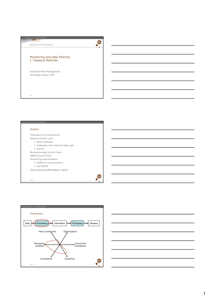
  1. Monitoring and data filtering I. Classical Methods Advanced Herd Management Dan Børge Jensen, IPH Dias 1 Outline Framework and Introduction Shewart Control chart • Basic principles • Examples: milk yield and daily gain • Alarms Moving Average Control Chart EWMA Control Chart Monitoring autocorrelation • Model for autocorrelation • Use EWMA Final exercises/Mandatory report Dias 2 Framework Herd constraints Optimization Biological Functional variation limitations Uncertainty Dynamics Dias 3 1

  2. Class Question: what’s going on, and what to do? (2 minutes) Average daily weight gain, Pig herds Results from 2 herds 880 870 860 850 840 Gain (g) 830 820 810 800 790 780 0 2 4 6 8 10 12 Quarter Expected Herd A Herd B Is the conclusion the same in both herds? Dias 4 Introduction (2/3) So far Control: compare key figures (k) with expected results κ = θ + e s + e o Deviation: see if significant from a statistical point of view If deviation: adjustement plan or/and implementation Problem: we assume that results can be evaluated without considering results from the previous period Dias 5 Introduction (3/3) Key figures regarded as a time series of observations, treated as a whole How to model the results? κ t = θ + e st + e ot = θ + ν t κ t : observed value of the key figure θ : true underlying value e st : sample error (biological variation) e ot : observation error (observation method) Dias 6 2

  3. Exercise 7.1.1 (10 minutes) Dias 7 The Shewart Control Chart: basic principles (1/2) Sample quality characteristic Upper Control Limit (UCL) κ 1 , κ 2 , ... κ n Center Line θ' Lower Control Limit (LCL) Sample number, or time Here: all the points fall inside the CL. Process in control Dias 8 The Shewart Control Chart: basic principles (2/2) Center line = target value • CL = θ’ Determination of the control limits • UCL t = θ’ + a σ t • LCL t = θ’ - a σ t We test the null hypothesis H 0 : θ’ = θ • a = 2 corresponds to approx. 5% precision level Usually distance parameter a = 2 or 3 • If a = 2 : ”2-sigma” control limit Dias 9 3

  4. Example 7.1: average daily milk yield – I’ll show you! (”Advanced topics”, page 45) Target value: CL = θ’ = 25.60 kg ECM for first lactation cows Overall herd SD over 24 weeks: 490 kg milk - But our ECM is considered at a daily level! N.Cows at beginning: 225 Control limits: UCL t = θ’ + a σ t 7 days per week LCL t = θ’ - a σ t Standard deviation calculated according to number of cows behind the average Dias 10 Example 1: milk yield Shewart control chart, 2-sigma CL N.Cows at beginning: 225  σ 1 = 0.194  2* σ 1 = 0.39 Dias 11 Exercise 7.1.2 (15 minutes) Dias 12 4

  5. Control and warning limits (1/3) UCL and LCL determined by a (e.g. a=2 <-> p=0.05) Choice of significance level / distance parameter: tradeoff between number of False Positives and False Negatives! Possible Scenarios: Low a High a Alarm Alarm Alarm No Alarm No Alarm No Alarm Type II Error System System System True True False HAS changed HAS changed HAS changed Positive Positive Negative System has NOT System has NOT System has NOT False True True changed changed changed Positive Negative Negative Type I Error Dias 13 Class Questions (5 minutes): If you have a HIGH observation frequency ( e.g. every hour or every second ) which sort of error should you MINIMIZE? And why? If you have a very LOW observation frequency ( e.g. every quarter or every year ) which sort of error should you MINIMIZE? And why? Alarm Alarm No Alarm No Alarm Alarm No Alarm System System True System True False HAS changed HAS changed Positive HAS changed Positive Negative System has NOT System has NOT True System has NOT False True changed changed Negative changed Positive Negative Dias 14 Control and warning limits (2/3) Sampling Frequency The more frequent κ is calculated, the higher a should be Average Run Length ARL =1/ q ARL: expected number of obs between 2 out-of-control alarms. q: the probability of an arbitrary point exceeding the control limits Average Time to Signal ATS =ARL/ ν v: sampling frequency, defined as observations per time unit Dias 15 5
  6. Control and warning limits (2.1/3) Example: Process in control  q = p a = 2  p = 0.05 ARL 0 = 1/ q = 1/ p = 1/0.05 = 20 Obs/Alarm Quaterly obs ATS 0 = ARL 0 / ν Two obs per second ATS 0 = ARL 0 / ν Dias 16 Control and warning limits (3/3) What is the cost of a What is the cost of a False Negative? False Positive? Alternative: use of warning limits Dias 17 Pattern detection What do we detect? - Level change, outliers, increase in variation (c ontrol limits) - Trend (increase, decrease), cyclic pattern, autocorrelation Rules of thumb (Montgomery, 2005): 1- One point outside the 3-Sigma limits 2- Two out of three consecutive points outside 2-Sigma limits 3- Four out of five consecutive points outside the 1-Sigma limit 4- Eight consecutive points on the same side of the expected level Dias 18 6

  7. Illustration of pattern detection From Example 1 ! Rule 4 Dias 19 5 Minute Break Dias 20 Example 2: daily gain of growing pigs Target value: θ’ = CL = 775 g Precision estimates ( σ ) Random sampling: 20.2 g Control limits: UCL = 775 + a σ, a = 2 LCL = 775 − a σ, a = 2 Dias 21 7

  8. Example 2: daily gain of growing pigs Shewart control chart, 2-sigma CL Dias 22 Example 2: daily gain of growing pigs Process out of control 8 obs out of 16 Seasonnal variation is to be expected in slaughter pig production If there is an expected pattern: use of other monitoring techniques to take it into account e.g. other classical techniques (presented next) or state space models (chapter 8) If no expected pattern: further analysis / intervention Dias 23 Moving Average Control Charts (1/2) The moving average is the average of the most recent n observations κ + + κ + κ σ K t ≥ 2 = − + − n t n 1 t 1 t with variance M ( n ) , t n n E.g. n = 4 M7(n) = 750 M6(n) = 744 M5(n) = 756 M4(n) = 763 Dias 24 8

  9. Moving Average Control Charts (2/2) Using n=4, a=3 What can we conclude? Dias 25 Exponentially Weighted Moving Average control charts (1/3) The EWMA is a weighted average of all observations until now = λκ + − λ ( 1 ) z z − t t t 1 λ   with variance, for large t, σ ≈ σ   2 2 z − λ   t 2 The most recent observations are always given highest weights The EWMA control chart is built the same way as the Shewart control chart Dias 26 Exponentially Weighted Moving Average control charts (2/3) First lactation, a=2, λ=0.68 Dias 27 9

  10. Exponentially Weighted Moving Average control charts (3/3) Choice of lambda: Small values favor detection of small shifts of θ ! Can take time to detect : small lambda = low weight to new obs Shewart control chart is suggested for detecting large shifts Combination of EWMA + Shewart for both small and large shifts Dias 28 Exercise 7.1.3 (15 minutes) Hints: k 1 = k[1] z t = z[t] z t-1 = z[t-1] Dias 29 Check for autocorrelation - Milk Yield example Present versus previous observation Sample autocorrelation Positive autocorrelation First lactation First lactation milk yields First lactation milk yields Dias 30 10

  11. A model for autocorrelation Model Predict next obs. Errors = Observed - predicted e , e ,..., e 1 2 t Forecast error Variance Forecast error Control chart! Dias 31 Control chart – correlated data The point of a model: IF “everything is fine” THEN “things progress as expected” Therefore: IF “things progress UN-expectedly” THEN “Something is wrong!” Dias 32 EWMA for autocorrelated data Use EWMA as one-step-ahead predictor for autocorrelated data κ ≈ ˆ z + 1 t t Choose λ by minimizing the sum of the squared forecast errors t = κ −  e z 2 e − t t t 1 i = i 1 The variance of the forecast errors is calculated as  = t 2 e σ = i 2 i 1 e t Dias 33 11

  12. Concluding remarks We have shifted focus from observing a key figure κ at time t to an entire time series (κ 1 , κ 2 ,... κ t ) We tried to detect changes in process (alarms) - Raw data (Shewart control chart) - Averaged data (Moving / Exponentially Moving Average) We observed autocorrelation: model, e.g. EWMA We observed seasonality Next time: classical time-series monitoring of categorical data! Dias 34 Break and exercises, until 17:00 Dias 35 12

Download Presentation
Download Policy: The content available on the website is offered to you 'AS IS' for your personal information and use only. It cannot be commercialized, licensed, or distributed on other websites without prior consent from the author. To download a presentation, simply click this link. If you encounter any difficulties during the download process, it's possible that the publisher has removed the file from their server.

Recommend


More recommend