[PDF] - 1 Real Neural Learning Artificial Neuron Model Model network as a PDF Document

SLIDE 1

1

CS 391L: Machine Learning Neural Networks Raymond J. Mooney

University of Texas at Austin

2

Neural Networks

Analogy to biological neural systems, the most

robust learning systems we know.

Attempt to understand natural biological systems

through computational modeling.

Massive parallelism allows for computational

efficiency.

Help understand “distributed” nature of neural

representations (rather than “localist” representation) that allow robustness and graceful degradation.

Intelligent behavior as an “emergent” property of

large number of simple units rather than from explicitly encoded symbolic rules and algorithms.

3

Neural Speed Constraints

Neurons have a “switching time” on the order of a

few milliseconds, compared to nanoseconds for current computing hardware.

However, neural systems can perform complex

cognitive tasks (vision, speech understanding) in tenths of a second.

Only time for performing 100 serial steps in this

time frame, compared to orders of magnitude more for current computers.

Must be exploiting “massive parallelism.”
Human brain has about 1011 neurons with an

average of 104 connections each.

4

Neural Network Learning

Learning approach based on modeling

adaptation in biological neural systems.

Perceptron: Initial algorithm for learning

simple neural networks (single layer) developed in the 1950’s.

Backpropagation: More complex algorithm

for learning multi-layer neural networks developed in the 1980’s.

5

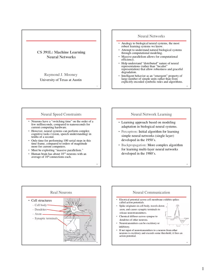
Real Neurons

Cell structures

– Cell body – Dendrites – Axon – Synaptic terminals

6

Neural Communication

Electrical potential across cell membrane exhibits spikes

called action potentials.

Spike originates in cell body, travels down

axon, and causes synaptic terminals to release neurotransmitters.

Chemical diffuses across synapse to

dendrites of other neurons.

Neurotransmitters can be excititory or

inhibitory.

If net input of neurotransmitters to a neuron from other

neurons is excititory and exceeds some threshold, it fires an action potential.

SLIDE 2

2

7

Real Neural Learning

Synapses change size and strength with

experience.

Hebbian learning: When two connected

neurons are firing at the same time, the strength of the synapse between them increases.

“Neurons that fire together, wire together.”

8

Artificial Neuron Model

Model network as a graph with cells as nodes and synaptic

connections as weighted edges from node i to node j, wji

Model net input to cell as
Cell output is:

1 3 2 5 4 6 w12 w13 w14 w15 w16

i i ji j

w

net

∑

=

(Tj is threshold for unit j)

j i j j j

T net T net

≥

< = if 1 if

netj

j

Tj 1

9

Neural Computation

McCollough and Pitts (1943) showed how such model

neurons could compute logical functions and be used to construct finite-state machines.

Can be used to simulate logic gates:

– AND: Let all wji be Tj/n, where n is the number of inputs. – OR: Let all wji be Tj – NOT: Let threshold be 0, single input with a negative weight.

Can build arbitrary logic circuits, sequential machines, and

computers with such gates.

Given negated inputs, two layer network can compute any

boolean function using a two level AND-OR network.

10

Perceptron Training

Assume supervised training examples

giving the desired output for a unit given a set of known input activations.

Learn synaptic weights so that unit

produces the correct output for each example.

Perceptron uses iterative update algorithm

to learn a correct set of weights.

11

Perceptron Learning Rule

Update weights by:

where η is the “learning rate” tj is the teacher specified output for unit j.

Equivalent to rules:

– If output is correct do nothing. – If output is high, lower weights on active inputs – If output is low, increase weights on active inputs

Also adjust threshold to compensate:

i j j ji ji

t

w w ) ( − + = η

) (

j j j j

t

T T − − = η

12

Perceptron Learning Algorithm

Iteratively update weights until convergence.
Each execution of the outer loop is typically

called an epoch.

Initialize weights to random values Until outputs of all training examples are correct For each training pair, E, do: Compute current output oj for E given its inputs Compare current output to target value, tj , for E Update synaptic weights and threshold using learning rule

SLIDE 3

3

13

Perceptron as a Linear Separator

Since perceptron uses linear threshold function, it is

searching for a linear separator that discriminates the classes.

1 3 13 2 12

T

w
w

> +

3
2

13 1 2 13 12 3

w T

w

w

+

− >

??

Or hyperplane in n-dimensional space

14

Concept Perceptron Cannot Learn

Cannot learn exclusive-or, or parity

function in general.

3
2

?? +

1 1

– + –

15

Perceptron Limits

System obviously cannot learn concepts it

cannot represent.

Minksy and Papert (1969) wrote a book

analyzing the perceptron and demonstrating many functions it could not learn.

These results discouraged further research
n neural nets; and symbolic AI became the

dominate paradigm.

16

Perceptron Convergence and Cycling Theorems

Perceptron convergence theorem: If the data is

linearly separable and therefore a set of weights exist that are consistent with the data, then the Perceptron algorithm will eventually converge to a consistent set of weights.

Perceptron cycling theorem: If the data is not

linearly separable, the Perceptron algorithm will eventually repeat a set of weights and threshold at the end of some epoch and therefore enter an infinite loop.

– By checking for repeated weights+threshold, one can guarantee termination with either a positive or negative result.

17

Perceptron as Hill Climbing

The hypothesis space being search is a set of weights and a

threshold.

Objective is to minimize classification error on the training set.
Perceptron effectively does hill-climbing (gradient descent) in

this space, changing the weights a small amount at each point to decrease training set error.

For a single model neuron, the space is well behaved with a

single minima. weights training error

18

Perceptron Performance

Linear threshold functions are restrictive (high bias) but

still reasonably expressive; more general than:

– Pure conjunctive – Pure disjunctive – M-of-N (at least M of a specified set of N features must be present)

In practice, converges fairly quickly for linearly separable

data.

Can effectively use even incompletely converged results

when only a few outliers are misclassified.

Experimentally, Perceptron does quite well on many

benchmark data sets.

SLIDE 4

4

19

Multi-Layer Networks

Multi-layer networks can represent arbitrary functions, but

an effective learning algorithm for such networks was thought to be difficult.

A typical multi-layer network consists of an input, hidden

and output layer, each fully connected to the next, with activation feeding forward.

The weights determine the function computed. Given an

arbitrary number of hidden units, any boolean function can be computed with a single hidden layer.

utput

hidden input activation

20

Hill-Climbing in Multi-Layer Nets

Since “greed is good” perhaps hill-climbing can be used to

learn multi-layer networks in practice although its theoretical limits are clear.

However, to do gradient descent, we need the output of a

unit to be a differentiable function of its input and weights.

Standard linear threshold function is not differentiable at

the threshold.

netj

i

Tj 1

21

Differentiable Output Function

Need non-linear output function to move beyond linear

functions.

– A multi-layer linear network is still linear.

Standard solution is to use the non-linear, differentiable

sigmoidal “logistic” function:

netj Tj 1 ) (

1 1

j j T

net j

e

−

−

+ =

Can also use tanh or Gaussian output function

22

Gradient Descent

Define objective to minimize error:

where D is the set of training examples, K is the set of

utput units, tkd and okd are, respectively, the teacher and

current output for unit k for example d.

The derivative of a sigmoid unit with respect to net input is:
Learning rule to change weights to minimize error is:

2

) ( ) (

kd D d K k kd

t

W E − = ∑∑

∈ ∈

) 1 (

j j j j

net
−

= ∂ ∂

ji ji

w E w ∂ ∂ − = ∆ η

23

Backpropagation Learning Rule

Each weight changed by:

where η is a constant called the learning rate tj is the correct teacher output for unit j δj is the error measure for unit j

i j ji

w

ηδ = ∆

unit

utput

an is if ) )( 1 ( j

t
j

j j j j

− − = δ unit hidden a is if ) 1 ( j w

k

kj k j j j

∑

− = δ δ

24

Error Backpropagation

First calculate error of output units and use this to

change the top layer of weights.

utput

hidden input Current output: oj=0.2 Correct output: tj=1.0 Error δj = oj(1–oj)(tj–oj) 0.2(1–0.2)(1–0.2)=0.128 Update weights into j

i j ji

w

ηδ = ∆

SLIDE 5

5

25

Error Backpropagation

Next calculate error for hidden units based on

errors on the output units it feeds into.

utput

hidden input

∑

− =

k kj k j j j

w

δ

δ ) 1 (

26

Error Backpropagation

Finally update bottom layer of weights based on

errors calculated for hidden units.

utput

hidden input

∑

− =

k kj k j j j

w

δ

δ ) 1 ( Update weights into j

i j ji

w

ηδ = ∆

27

Backpropagation Training Algorithm

Create the 3-layer network with H hidden units with full connectivity between layers. Set weights to small random real values. Until all training examples produce the correct value (within ε), or mean squared error ceases to decrease, or other termination criteria: Begin epoch For each training example, d, do: Calculate network output for d’s input values Compute error between current output and correct output for d Update weights by backpropagating error and using learning rule End epoch

28

Comments on Training Algorithm

Not guaranteed to converge to zero training error,

may converge to local optima or oscillate indefinitely.

However, in practice, does converge to low error

for many large networks on real data.

Many epochs (thousands) may be required, hours
r days of training for large networks.
To avoid local-minima problems, run several trials

starting with different random weights (random restarts).

– Take results of trial with lowest training set error. – Build a committee of results from multiple trials (possibly weighting votes by training set accuracy).

29

Representational Power

Boolean functions: Any boolean function can be

represented by a two-layer network with sufficient hidden units.

Continuous functions: Any bounded continuous

function can be approximated with arbitrarily small error by a two-layer network.

– Sigmoid functions can act as a set of basis functions for composing more complex functions, like sine waves in Fourier analysis.

Arbitrary function: Any function can be

approximated to arbitrary accuracy by a three- layer network.

30

Sample Learned XOR Network

3.11 −7.38 6.96 −5.24 −3.6 −3.58 −5.57 −5.74 −2.03

A X Y B Hidden Unit A represents: ¬(X ∧ Y) Hidden Unit B represents: ¬(X ∨ Y) Output O represents: A ∧ ¬B = ¬(X ∧ Y) ∧ (X ∨ Y) = X ⊕ Y O

SLIDE 6

6

31

Hidden Unit Representations

Trained hidden units can be seen as newly

constructed features that make the target concept linearly separable in the transformed space.

On many real domains, hidden units can be

interpreted as representing meaningful features such as vowel detectors or edge detectors, etc..

However, the hidden layer can also become a

distributed representation of the input in which each individual unit is not easily interpretable as a meaningful feature.

32

Over-Training Prevention

Running too many epochs can result in over-fitting.
Keep a hold-out validation set and test accuracy on it after

every epoch. Stop training when additional epochs actually increase validation error.

To avoid losing training data for validation:

– Use internal 10-fold CV on the training set to compute the average number of epochs that maximizes generalization accuracy. – Train final network on complete training set for this many epochs. error

n training data
n test data

# training epochs

33

Determining the Best Number of Hidden Units

Too few hidden units prevents the network from

adequately fitting the data.

Too many hidden units can result in over-fitting.
Use internal cross-validation to empirically determine an
ptimal number of hidden units.

error

n training data
n test data

# hidden units

34

Successful Applications

Text to Speech (NetTalk)
Fraud detection
Financial Applications

– HNC (eventually bought by Fair Isaac)

Chemical Plant Control

– Pavillion Technologies

Automated Vehicles
Game Playing

– Neurogammon

Handwriting recognition

35

Issues in Neural Nets

More efficient training methods:

– Quickprop – Conjugate gradient (exploits 2nd derivative)

Learning the proper network architecture:

– Grow network until able to fit data

Cascade Correlation
Upstart

– Shrink large network until unable to fit data

Optimal Brain Damage
Recurrent networks that use feedback and can

learn finite state machines with “backpropagation through time.”

36

Issues in Neural Nets (cont.)

More biologically plausible learning

algorithms based on Hebbian learning.

Unsupervised Learning

– Self-Organizing Feature Maps (SOMs)

Reinforcement Learning

– Frequently used as function approximators for learning value functions.

Neuroevolution